Metrics in a moving window

A landscape metric gives one number for a whole map. But a region of 50 km is rarely uniform: there are open plains, a mosaic of fields and woods, a city. A moving window computes the metric for the neighbourhood of every cell and writes it on that cell, so the number becomes a map: where is the landscape diverse, where is it full of edges, where is it homogeneous? This part runs metrics.window on CORINE Land Cover around Hannover in Germany, shows with a slider how the size of the window changes the answer, compares square and circular windows, and explains how to choose the window from the question. At the end you will have maps of landscape structure you can use as predictors or to plan, and you will know how to justify their scale.

The idea#

Slide a square of \(w \times w\) cells over the map. At every position, treat the cells inside it as a landscape of its own, compute a landscape metric, and write the value on the cell at the centre. Repeat for every cell: the result is a map of the metric at the scale of the window. The idea is old in remote sensing (texture filters) and was brought to landscape ecology to map forest fragmentation over continents (Riitters et al., 2000), then generalised to any metric (Hagen-Zanker, 2016); landscapemetrics' window_lsm (Hesselbarth et al., 2019) does it for its landscape metrics, and Terraflux's metrics.window does the same.

Key idea: a metric at a scale

The window's size is the scale of the map you get. A window of \(w\) cells of side \(c\) metres covers \((w c)^2\) m²: 21 cells of 100 m is a square of 2.1 km, 441 ha. Every value on the map answers "what is the landscape like within about \(w c / 2\) of here?". A small window sees the immediate surroundings and changes abruptly from cell to cell; a large window sees a wide area and changes smoothly. Neither is right in general: the window should match the distance at which the landscape matters to the process you study.

Every landscape-level metric can be computed in a window: diversity, edge density, contagion, richness, the number of patches. Class-level metrics are not computed directly; for the share of one class around every cell, use GuidosToolbox's density (fragmentation) or reclassify the map to that class and another first.

When to use it#

Mapping heterogeneity for planning or description: where the farmed landscape is a diverse mosaic and where it is a uniform plain.
Predictors for a species model: the diversity or edge density around every cell as a layer for a species distribution model, at the scale the species perceives.
Finding transitions between kinds of landscape, which a single number for the whole map hides.
Not when you have sites and want the landscape around each: computing only those windows is faster and gives a table (part 5, metrics.sample). And not when you want kinds of landscape with defined boundaries: tiles of a grid are easier to classify (part 6).

What you need#

A categorical map in a projected system. We use clc.tif, CORINE Land Cover around Hannover: 2,000 × 2,000 cells of 25 m (50 × 50 km) in the European equal-area system (EPSG:3035), with CORINE's classes of level 3. We group them into 7 broad classes and resample to 100 m, which keeps the windows fast and corresponds to CORINE's minimum mapping unit of 25 ha (a square of 500 m) better than 25 m does.

In the application, Templates > Landscape metrics > Landscape metrics has a metrics.window node with Shannon's diversity and edge density in a window of 9 cells.

Build the model#

CORINE grouped into 7 classes, at 100 m, and three landscape metrics in a window of 21 cells (2.1 km) around every cell.

Model file (TOML)

format = "terraflux/1"

[[nodes]]
id = "corine"
op = "raster.read"
params = { path = "clc.tif" }
note = "CORINE Land Cover, 25 m."

[[nodes]]
id = "broad"
op = "raster.reclassify"
inputs = { map = "corine.raster" }
params = { rules = "1..11 -> 1\n12 -> 2\n13..22 -> 3\n23..25 -> 4\n26..34 -> 5\n35..39 -> 6\n40..44 -> 7" }
note = "Urban, arable, pasture and mixed farming, forest, heath and grass, wetlands, water."

[[nodes]]
id = "cover"
op = "raster.resample"
inputs = { raster = "broad.map" }
params = { resolution = 100, resampling = "mode" }
note = "100 m: the most common class of each 4 x 4 cells."

[[nodes]]
id = "window"
op = "metrics.window"
inputs = { map = "cover.raster" }
params = { metrics = ["shdi", "ed", "pr"], window = 21 }
note = "A map per metric."

[[plots]]
id = "plot"
title = "Around every cell"
layers = [{ from = "window.maps" }]

Read and group the classes (nodes 1 and 2). raster.reclassify takes a rule per line; 1..11 -> 1 puts CORINE's classes 1 to 11 (artificial surfaces) in class 1, and so on. Fewer classes make a diversity that means something: with 44 classes, diversity mostly counts the mappers' distinctions.
Coarsen the grain (node 3). raster.resample with resolution = 100 and resampling = "mode" gives every new cell the most common class of the 16 cells it covers. Connect node 2's map to its raster input.
The window (node 4). Click metrics.window in the library's Landscape metrics and connect node 3's raster to its map input. metrics lists the landscape metrics, window the side in cells (odd, so that the window has a centre; default 5), shape square (default) or circle.
Look. Click node 4: the Viewer shows its output maps, a stack with a map per metric named after it; pick the layer in the Viewer. To keep the view with the model, choose Plots › Save as a new plot and give it a title (here Around every cell).

A window of 21 cells over a map of 500 × 500 is 250,000 small landscapes, each of 441 cells: a few seconds. The time grows with the window's area, so windows of hundreds of cells on large maps take long; part 7 runs them by strips of rows on maps larger than memory.

Read the results#

CORINE Land Cover in seven classes — CORINE Land Cover around Hannover (50 × 50 km) in seven broad classes at 100 m: arable land covers half of it, forest a fifth, the city of Hannover (red) the east, the lake Steinhuder Meer (blue) the north-west.

Shannon's diversity in a window of 21 cells — Shannon's diversity within 2.1 km of every cell. The highest values (yellow) are where farmland, forest, pasture and settlements meet, as around the lake; the lowest (dark) are the large uniform areas: the open plains in the south, the centre of the city in the east, the interior of the large forests.

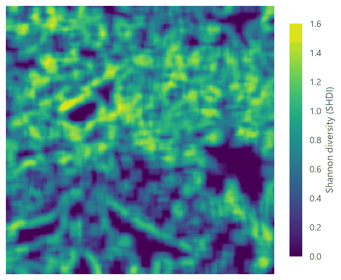
Read the diversity map against the land cover: the dark areas are not "poor" landscapes but uniform ones at this scale, a city centre as much as a plain of fields. The edge density map tells a similar story with a different emphasis: it is high where patches are small, whatever their classes.

Settings that change the answer: the window's size#

Move the slider from windows of 3 cells (300 m) to 41 cells (4.1 km).

Window side (cells of 100 m) 3 — Shannon's diversity of the window around every cell, from 3 to 41 cells. Small windows draw the boundaries between patches: most cells see one class (diversity 0, dark). Large windows draw regions: the mosaic around the lake and the plains in the south. Numbers: the mean diversity over the map, and the share of cells whose window holds only one class.

Window side (cells of 100 m) 5 — Shannon's diversity of the window around every cell, from 3 to 41 cells. Small windows draw the boundaries between patches: most cells see one class (diversity 0, dark). Large windows draw regions: the mosaic around the lake and the plains in the south. Numbers: the mean diversity over the map, and the share of cells whose window holds only one class.

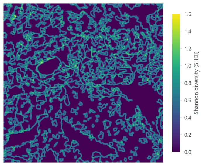
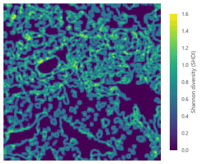
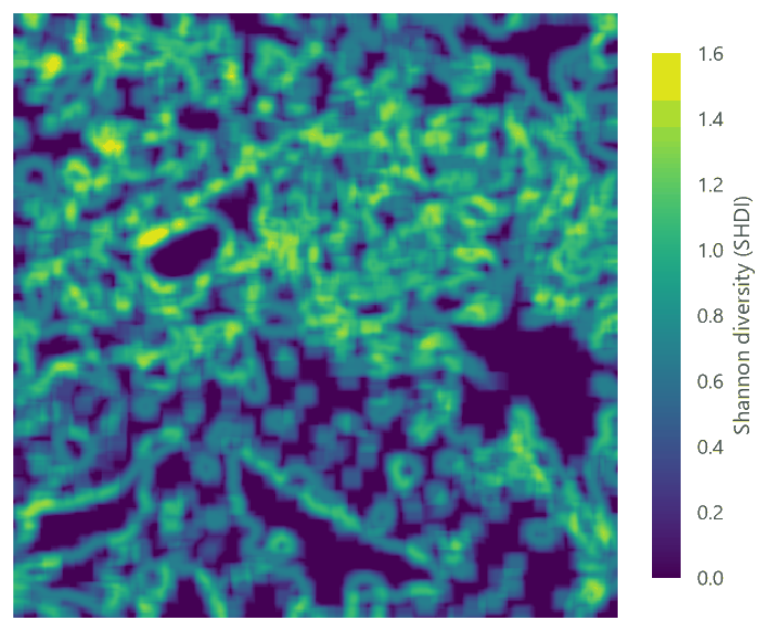
Three things happen as the window grows:

The values rise. A larger window holds more classes (from 1.3 on average to 3.9), so diversity rises: the mean SHDI goes from 0.18 to 0.90. A diversity of 0.7 means "diverse" in a window of 2 km and "uniform" in one of 10 km. Values computed with different windows cannot be compared.
The map smooths. Neighbouring windows share most of their cells, so the map varies more slowly; the differences between places shrink once the window is larger than the typical patch. The spread of SHDI across cells (its SD) peaks at about 15 cells and then falls.
The pattern changes meaning. At 3 cells the map draws the boundaries between patches; at 41 it draws regions. In between, at the windows of 9 to 21 cells, it shows the mosaics of fields and woods.

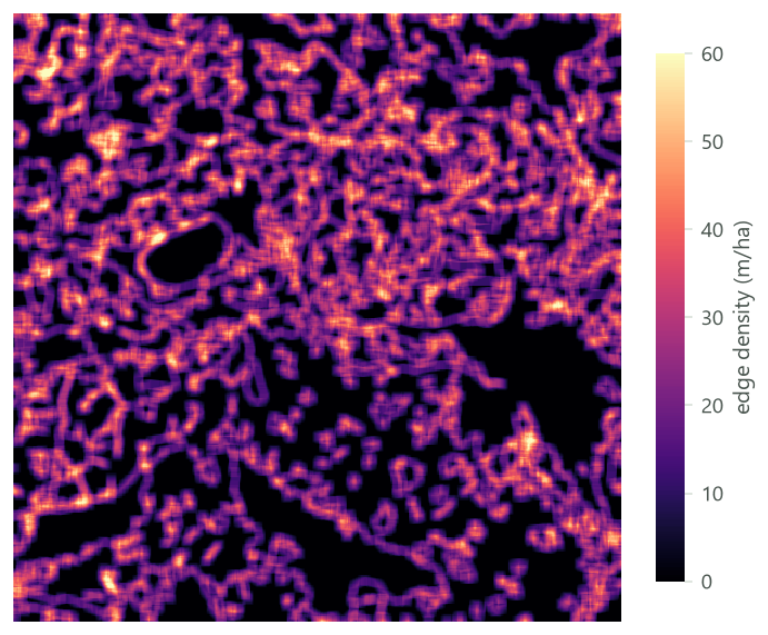
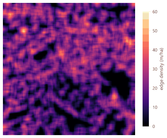
The edge density does the same, with one more effect:

Choosing the window#

Choose the window from the ecology, then check the sensitivity:

From the organism: its home range, its daily movements, its dispersal distance. A window whose side is about twice the distance over which the landscape affects the species: for a ground beetle, a few hundred metres; for a bird of farmland, one or two kilometres; for a large mammal, tens of kilometres.
From the data: when the species' scale is unknown, compute the windows at several sizes and let the data choose the one that best explains the response: the scale of effect (Jackson & Fahrig, 2015), tested in part 5 with plots of several radii.
From the map: a window should hold many cells (at least a few dozen) for the metric to be stable, and its cells should be much smaller than the window: below 5 cells, a window sees mostly one or two patches.

Which metrics to put in a window#

Any landscape-level metric works, but they do not all mean the same thing inside a window:

Composition (pr, shdi, sidi, shei): the variety of land covers within reach. These are the most robust in windows: they depend only on the counts of cells.
Edges and adjacencies (ed, contag, ai, iji, and the information-theory metrics ent, condent, mutinf): how fine-grained the mosaic is around each cell. They count pairs of cells inside the window, so they too are well defined, with the caveat of the window's own border (the edges along it are not counted).
Patch-based metrics (np, area_mn, lpi, shape_mn...): the patches are those cut by the window. A forest of 1,000 ha seen through a window of 441 ha is a patch of at most 441 ha; area_mn in a window measures the pieces of patches the window holds, not the patches. Use them with care, and only with windows much larger than the typical patch.

For the share of one class around every cell (the forest within 1 km, say), the window of a landscape metric is the wrong tool: GuidosToolbox's density (fragmentation.fad, on the forest cells) or a share computed by map algebra answer it directly (fragmentation).

In the literature

Riitters et al. (2000) mapped the world's forest fragmentation with moving windows of several sizes, and found that the picture of the world's forests changes with the size of the window: there is no single scale at which forest is fragmented or not. Hagen-Zanker (2016) showed how to compute windows of any metric quickly for very large maps, which is what makes windows of hundreds of cells practical today.

Square or circle#

shape = "circle" keeps only the cells within half the side of the centre: a disc, the same distance in every direction, as a buffer around a point. A square window of the same side covers 27% more area (its corners).

Prefer circles when the window stands for the distance a species moves in any direction; squares are faster and are what most published moving-window studies used. Either way, say which.

Report it

Report the metric, the window's side in cells and in metres, its shape, the map's grain and legend, and how the border of the map was treated. Near the border a window is cut and holds fewer cells: there the values rest on less of the landscape. Either clip the result by half a window, or compute it on a map larger than the study area.

Common pitfalls#

Comparing maps of different windows, above.
A window smaller than the patches. Most windows then see one class and the map is mostly zero. Coarsen the grain or enlarge the window.
Using a window map as independent data. Neighbouring cells share most of their window, so their values are strongly autocorrelated; a statistical model that treats every cell as independent overstates the evidence. Sample the map at points far enough apart, or model the autocorrelation.
Edge density in small windows. It is underestimated (above), and it depends strongly on the grain.
Too many classes. In a window of a few hundred cells, 44 CORINE classes give diversity values driven by rare classes. Group the classes to those that matter for the question.

Going further#

Part 5: metrics around sites at several radii, through time, and their correlation.
Part 7: moving windows on maps larger than memory.
Fragmentation: GuidosToolbox's moving windows of one habitat (density, contagion, entropy) at several scales.
Surface metrics: windows over continuous surfaces.
The operator reference: metrics.window.

References#

Hagen-Zanker, A. (2016). A computational framework for generalized moving windows and its application to landscape pattern analysis. International Journal of Applied Earth Observation and Geoinformation, 44, 205–216. https://doi.org/10.1016/j.jag.2015.09.010
Hesselbarth, M. H. K., Sciaini, M., With, K. A., Wiegand, K., & Nowosad, J. (2019). landscapemetrics: an open-source R tool to calculate landscape metrics. Ecography, 42(10), 1648–1657. https://doi.org/10.1111/ecog.04617
Jackson, H. B., & Fahrig, L. (2015). Are ecologists conducting research at the optimal scale? Global Ecology and Biogeography, 24(1), 52–63. https://doi.org/10.1111/geb.12233
Riitters, K., Wickham, J., O'Neill, R., Jones, B., & Smith, E. (2000). Global-scale patterns of forest fragmentation. Conservation Ecology, 4(2), 3. https://doi.org/10.5751/ES-00209-040203