Circuitscape: currents between forests

With the ideas of part 1 and the resistance of part 2, you can now run Circuitscape on a real landscape. You will connect the eight largest forests around Hannover in Circuitscape's four modes, each answering a different question: how isolated is every pair of forests (pairwise), how connected is each forest to all the others (one-to-all and all-to-one), and where would animals leaving one forest go (advanced). You will read the matrix of effective resistances, find the pinch points on the current maps, and drag a handle between a least-cost corridor and the current between two forests to see what each shows. At the end you will be able to run Circuitscape's analyses in a Terraflux model, and know which mode fits which question.

The idea#

Circuitscape's four modes#

Circuitscape (McRae et al., 2008; Anantharaman et al., 2020) solves the circuit of a raster: every cell is a node joined to its neighbours. The modes differ in where current enters and where it leaves:

Mode	Current enters	Current leaves	Question
Pairwise	each focal area in turn (1 A)	another focal area	How isolated is each pair? Where does movement between them go?
One-to-all	one focal area (1 A)	all the others (grounded)	How connected is each area to the rest?
All-to-one	all the other areas (1 A each)	one area	Where does movement towards an area come from?
Advanced	any cells (a source map)	any cells (a ground map)	Free: any sources, sinks and strengths

In pairwise mode, the cumulative current map (cum) adds up the currents of all pairs: a cell bright on it carries movement between many pairs. The maximum current map (max) keeps, for each cell, its largest current of any pair: it shows routes important to even one pair.

Key idea: pinch points and current density

The current through a cell is the share of the movement between the focal areas that passes there (for 1 A injected). Where the landscape funnels movement into a narrow passage, every route crowds into a few cells and their current rises: a pinch point. Pinch points are where connectivity is most vulnerable (a little habitat lost there cuts a lot of movement) and where protection or restoration does the most. McRae et al. (2012) used current maps to find barriers whose removal would most improve connectivity, and Dickson et al. (2013) to map the pinch points of puma habitat across the south-western United States.

Effective resistance as distance#

The effective resistance between two areas (part 1) is their isolation over every route at once. It grows with distance, but also with the number and quality of routes: two forests joined by a broad band of pasture are closer, in resistance, than two equally distant forests joined by one narrow strip. McRae (2006) proposed it as a predictor of genetic distance between populations, isolation by resistance, and McRae and Beier (2007) showed that it outperformed straight and least-cost distances in two species.

When to use it#

Pairwise: comparing the isolation of populations or reserves; corridors between a few core areas; landscape genetics.
One-to-all: ranking areas by how connected they are to the rest of a network.
All-to-one: the catchment of an area, where animals reaching a reserve or a crossing come from.
Advanced: anything else, for example one source area spreading into a landscape with several sinks, or sources weighted by population size.

When the areas are not obvious (no reserves, a continuous habitat), use Omniscape instead.

What you need#

The class resistance of part 2, from clc_100m.tif.
Focal areas: here the eight forests of 1,500 ha or more, numbered as in the habitat networks series: 6, 8, 30, 45, 47, 55, 96 and 110. In your study they would be reserves, populations or sampling sites, as a raster of ids (0 or no value elsewhere).

The eight forests of 1,500 ha or more used as focal areas — The focal areas: the eight forests of 1,500 ha or more (dark green), with their numbers, over the land cover (pale). They ring the landscape: three in the south, two in the north-west, two in the north-east and one in the west.

The application's template Circuit connectivity (Templates > Connectivity) has the pairwise mode and Omniscape on a landscape drawn by chance.

Build the model#

1. The resistance and the focal areas#

The resistance is the raster.reclassify of part 2. The focal areas come from the forest patches: as before, conn.graph_from_raster and conn.nodes give the patches and their areas, two conn.to_map paint the areas and the ids on them, and a raster.calc keeps the large ones:

coalesce(p if a >= 1500 else 0, 0)

(a the area, p the patch id; coalesce turns "no value" outside the forests into 0).

2. The three focal modes#

circuit.pairwise, circuit.one_to_all (and a second circuit.one_to_all with all_to_one = true) take the resistance in habitat and the focal areas in points. Set cum_map = true (and max_map = true for pairwise) to get the maps. Each has a resistances table: for pairwise a matrix (a row per area, a column per area), for one-to-all one effective resistance per area. All-to-one measures no resistances: its table's value column is 0 for every area, as in Circuitscape, and its result is the current map.

The eight largest forests as focal areas, and Circuitscape's pairwise, one-to-all and all-to-one modes over the class resistance.

Model file (TOML)

format = "terraflux/1"

[[nodes]]
id = "land"
op = "raster.read"
params = { path = "clc_100m.tif" }

[[nodes]]
id = "resistance"
op = "raster.reclassify"
inputs = { map = "land.raster" }
params = { rules = "23 24 25 -> 1\n29 -> 2\n21 26 27 32 35 36 -> 5\n18 20 -> 10\n12 -> 20\n10 11 -> 30\n7 8 9 -> 50\n1 2 3 4 5 6 40 41 -> 100\n* -> 20" }

[[nodes]]
id = "graph"
op = "conn.graph_from_raster"
inputs = { map = "land.raster" }
params = { habitat = [23, 24, 25], area_unit = "ha" }

[[nodes]]
id = "patches"
op = "conn.nodes"
inputs = { map = "land.raster" }
params = { habitat = [23, 24, 25], area_unit = "ha" }

[[nodes]]
id = "area"
op = "conn.to_map"
inputs = { graph = "graph.graph", table = "patches.table" }
params = { column = "attribute" }

[[nodes]]
id = "patch"
op = "conn.to_map"
inputs = { graph = "graph.graph", table = "patches.table" }
params = { column = "id" }

[[nodes]]
id = "cores"
op = "raster.calc"
inputs = { a = "area.map", p = "patch.map" }
params = { expression = "coalesce(p if a >= 1500 else 0, 0)" }
note = "The forests of 1,500 ha or more, by number."

[[nodes]]
id = "pairwise"
op = "circuit.pairwise"
inputs = { habitat = "resistance.map", points = "cores.map" }
params = { cum_map = true, max_map = true }

[[nodes]]
id = "one_to_all"
op = "circuit.one_to_all"
inputs = { habitat = "resistance.map", points = "cores.map" }
params = { cum_map = true }

[[nodes]]
id = "all_to_one"
op = "circuit.one_to_all"
inputs = { habitat = "resistance.map", points = "cores.map" }
params = { cum_map = true, all_to_one = true }

3. The advanced mode#

circuit.advanced takes three maps: a conductance (1 / resistance, a raster.calc 1 / r), a source (the current injected at each cell, in amperes) and a ground (each cell's conductance to the ground: 0 none, 1 / 0, infinite, a direct ground). To ask where would animals leaving the southern forest go, if they settled in any of the other large forests, the source is 1 in every cell of forest 55 (1 if c == 55 else 0 on the cores) and the ground is infinite in the other seven (1 / 0 if c > 0 and c != 55 else 0). Its outputs are current and voltage.

The advanced mode: current injected over the southern forest, grounded in the seven others.

Model file (TOML)

[[nodes]]
id = "conductance"
op = "raster.calc"
inputs = { r = "resistance.map" }
params = { expression = "1 / r" }

[[nodes]]
id = "source"
op = "raster.calc"
inputs = { c = "cores.map" }
params = { expression = "1 if c == 55 else 0" }

[[nodes]]
id = "ground"
op = "raster.calc"
inputs = { c = "cores.map" }
params = { expression = "1 / 0 if c > 0 and c != 55 else 0" }

[[nodes]]
id = "advanced"
op = "circuit.advanced"
inputs = { conductance = "conductance.map", source = "source.map", ground = "ground.map" }

Circuitscape's own files

If you already have Circuitscape projects, circuit.circuitscape_ini runs an INI file as it is, with its inputs and options (polygons, masks, included pairs, variable source strengths), and writes the outputs as Circuitscape names them. Its results are the same as Circuitscape's: every solve is exact.

Read the results#

Effective resistances between the forests#

The matrix of effective resistances between the eight forests — Pairwise mode's resistances: the effective resistance between every pair of forests (ohms, for this resistance surface). The closest pair is 30 and 47 in the north-west (0.96), then 96 and 110 in the north-east (1.85) and 8 and 45 in the south-west (2.02); the most isolated is 45 to 110, across the whole landscape (8.46).

Effective resistance of the 28 pairs against the straight distance between their centres. They are strongly correlated (Pearson's r = 0.91): across this landscape of mostly arable land, distance explains most of the isolation. Above the trend (more isolated than their distance): the pairs of the western forest 6. Below it: the northern forests 30, 96 and 110, joined by the many woods of the north.

The effective resistances follow distance closely here (r = 0.91), as one would expect in a landscape whose matrix is mostly arable land. The interest lies in the departures. The western forest 6 is more isolated than its distances suggest (from 8 and 45 above all): open farmland surrounds it, with few routes. The forests of the north (30, 96, 110) are less isolated than their distances suggest: the small woods between them offer many cheap routes, and circuit theory counts every one. In a genetic study these are the pairs to look at, and the comparison of effective resistance, least cost and distance as predictors of genetic distance is the test McRae and Beier (2007) made.

Where movement goes: the pairwise current#

The cumulative current of the 28 pairs — The pairwise cumulative current: the currents of the 28 pairs of forests added (logarithmic; the focal forests in white). Bright channels run through the centre and north of the landscape, east of Lake Steinhude (the dark oval) and between the northern forests; the east, around Hannover, carries little.

The cumulative current shows the landscape's corridors: the bright channels follow woods, pastures and heaths, the cheaper land, and gather where they must pass between towns, the lake and open arable land. Look for two signs:

Bright, narrow bands between dark areas: pinch points, where many pairs' movement crowds into a few cells. The bright band just east of Lake Steinhude, squeezed between the lake and the towns, is the clearest here.
Broad, diffuse brightness: redundant routes, where losing one strip of habitat would be compensated by others.

Connected to the rest: one-to-all and all-to-one#

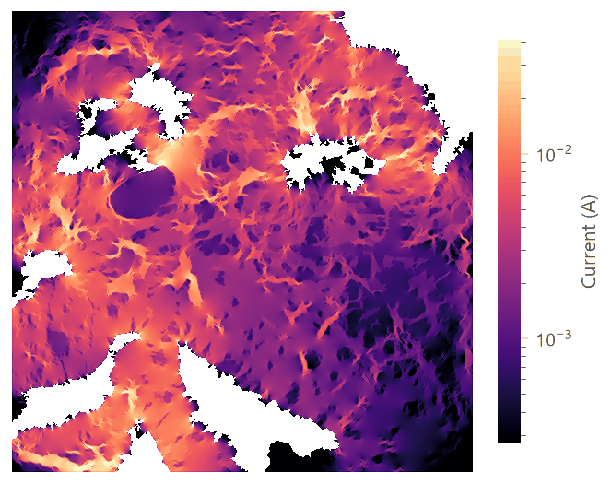
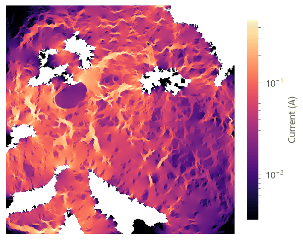
One-to-all's resistances rank the forests by their isolation from the rest of the network: 47 (0.80) and 30 (0.80), in the north-west, are the best connected; 96 (1.21) and 8 (1.36) next; 6 in the west (2.47) the most isolated. This ranking is the circuit-theory analogue of the importance of a patch in a habitat graph (part 3 of habitat networks), with all routes counted.

Spreading from one forest: the advanced mode#

Current spreading from the southern forest to the seven others — The advanced mode: current injected over every cell of the southern forest (1 A per cell), grounded in the seven other large forests (logarithmic). Most of it goes to the nearest forests, 8 and 45 in the south-west; a weaker stream runs north through the centre.

With every cell of forest 55 injecting 1 A, the current shows where dispersers leaving it would go if they kept moving until they reached another large forest: most to the near south-western forests, a share north through the woods of the centre. The voltage output gives, for every cell, the "pressure" of dispersers from the source: high near it, falling towards the grounds.

A least-cost corridor beside the current#

To compare, the same model computes a least-cost corridor between forest 55 and forest 96 with the grid distances operators: cost.transition makes the conductance between neighbours (function = "mean", reciprocal = true on the resistance), cost.geo_correction corrects it for the diagonals, cost.acc_cost gives the cost from each forest, and their sum, minus its least value, is how much dearer the best route through each cell is than the best route of all. Cells within a few percent of the least cost form the corridor. Drag the handle:

Current — Left: the least-cost corridor between the southern forest and forest 96 (bright: the route through the cell costs at most a few percent more than the best route; dark: 25% more or above). Right: Circuitscape's current between the same two forests (bright: most current, logarithmic). The corridor is one band north through the centre-west, then east; the current spreads over many routes and lights that band as only one of them.

The best route between the two forests costs 202,287 (in resistance × metres: as much as 10 km of arable land); 7,133 cells lie on routes within 5% of it, 14,771 within 10%. The corridor is one band: north from the southern forest through the woods of the centre-west, then east, past the lake, to forest 96. The current lights the same band, but also many others across the centre: many slightly dearer routes, together, carry much of the movement, and none of them appears on the corridor map. The effective resistance between the two forests, 5.36, sums up all of them.

In the literature

Report the resistance (values and sources), the focal areas, the mode, the connection scheme (8 neighbours, average conductance) and the software. Show the cumulative current with a stated colour scale (current maps are almost always shown with a logarithmic or quantile stretch), and name the pinch points. McRae et al. (2012) and Dickson et al. (2019) give examples and advice.

Settings that change the answer#

The resistance (part 2): the contrasts between classes sharpen or spread the current.
The focal areas: regions (all cells of a forest, as here) or single points. Points concentrate the current next to them, which shows as bright spots that are artefacts; regions spread it over their edge.
four_neighbors and avg_resistances: the connection scheme (part 1).
focal_zero: current set to 0 on the focal areas in the maps, so that they do not dominate the colour scale.
Polygons and masks (polygons, mask): short-circuit regions (cells joined at no cost, for example a reserve treated as one node) and cells left out of the circuit.

Common pitfalls#

Comparing current maps of different runs without normalising. Current depends on what is injected (1 A per pair, per area, or per cell in the advanced mode); compare shapes, or normalise.
Focal areas at the map's edge. Current cannot go around them, and the edge looks like a barrier. Buffer the study area (Koen et al., 2010).
Too many pairs. Pairwise mode solves one problem per area (and every pair with it); hundreds of areas are fine, thousands slow. For many areas, Omniscape or one-to-all is cheaper. One-to-all and all-to-one (as nodes, or in an INI file run by circuit.circuitscape_ini) solve the areas in batches (batch, by default four per thread) and tell how far they are in the application's status bar (one_to_all: one to all: 16 of 120 points); Stop stops them between two batches. Pairwise cannot stop in the middle of its solves: after Stop the run ends, and the node goes on in the background until it is done.
Effective resistance read as a probability. It is a distance, relative to the resistance surface; only its ranking and its correlation with other measures carry over between studies.

Going further#

Part 4: Omniscape: connectivity everywhere, without focal areas.
Grid distances: least-cost paths and corridors in more detail, and random walks between them.
Costs and corridors: what restoring a corridor gains.
The operators: circuit.pairwise, circuit.one_to_all, circuit.advanced, circuit.circuitscape_ini, circuit.network_pairwise, circuit.network_advanced.

References#

Anantharaman, R., Hall, K., Shah, V. B., & Edelman, A. (2020). Circuitscape in Julia: high performance connectivity modelling to support conservation decisions. JuliaCon Proceedings, 1(1), 58. https://doi.org/10.21105/jcon.00058
Dickson, B. G., Roemer, G. W., McRae, B. H., & Rundall, J. M. (2013). Models of regional habitat quality and connectivity for pumas (Puma concolor) in the southwestern United States. PLoS ONE, 8(12), e81898. https://doi.org/10.1371/journal.pone.0081898
Dickson, B. G., Albano, C. M., Anantharaman, R., Beier, P., Fargione, J., Graves, T. A., Gray, M. E., Hall, K. R., et al. (2019). Circuit-theory applications to connectivity science and conservation. Conservation Biology, 33(2), 239–249. https://doi.org/10.1111/cobi.13230
Koen, E. L., Garroway, C. J., Wilson, P. J., & Bowman, J. (2010). The effect of map boundary on estimates of landscape resistance to animal movement. PLoS ONE, 5(7), e11785. https://doi.org/10.1371/journal.pone.0011785
McRae, B. H. (2006). Isolation by resistance. Evolution, 60(8), 1551–1561. https://doi.org/10.1111/j.0014-3820.2006.tb00500.x
McRae, B. H., & Beier, P. (2007). Circuit theory predicts gene flow in plant and animal populations. Proceedings of the National Academy of Sciences, 104(50), 19885–19890. https://doi.org/10.1073/pnas.0706568104
McRae, B. H., Dickson, B. G., Keitt, T. H., & Shah, V. B. (2008). Using circuit theory to model connectivity in ecology, evolution, and conservation. Ecology, 89(10), 2712–2724. https://doi.org/10.1890/07-1861.1
McRae, B. H., Hall, S. A., Beier, P., & Theobald, D. M. (2012). Where to restore ecological connectivity? Detecting barriers and quantifying restoration benefits. PLoS ONE, 7(12), e52604. https://doi.org/10.1371/journal.pone.0052604