

Dynamic drivers and agents, part 1 of 4
Dynamic drivers: variables that move with the simulated map
Recompute a driver such as the distance to built land from the simulated map at every step, inside the loop, and see how that feedback changes where a model puts new land use.
- Level
- Intermediate
- Time
- 40 min
Most drivers of land change stay put while a model runs: the slope, the soil, the elevation of a cell do not change in fifteen years. Some drivers, though, are made of the land use itself: the distance to the nearest built-up cell, the share of forest around a cell, the distance to the nearest field. When the model builds a new house, the distance to built land changes for every cell around it. In this first part of the series you will make such a driver dynamic: you will compute it again from the simulated map at every step, put it back in the stack of drivers under the name the regressions know, and predict the suitability again before each allocation. You will run the same CLUE-S model on the Plum Island Ecosystems twice, once with the driver frozen in 1985 and once with it updated every year, and see what the feedback does to the pattern of new built land. At the end you will know how the nodes of a loop connect when a driver moves, which mistakes make a dynamic driver useless or misleading, and how to tell whether the feedback helps your model.
The idea#
Drivers that are made of land use#
A land change model decides where change goes from a map of suitability (or transition potential): for every cell, how likely each land use is, given the drivers, the explanatory variables such as slope or the distance to roads (see the foundations of land change models and suitability from logistic regressions). In CLUE-S (Verburg et al., 2002) the suitability of each class is a logistic regression on the drivers, fitted once on an observed map.
Some drivers describe the land use itself. Urban land grows next to urban land; fields are cleared next to fields; abandoned land returns to forest faster near a forest that can send seeds. Models of urban growth were built on this observation: in the cellular automata of White and Engelen (1993), the state of a cell's neighbourhood is the main driver of what the cell becomes. Verburg et al. (2004) showed how to measure such neighbourhood characteristics of land use and add them to the regressions of CLUE-S, so that a class becomes more suitable where it is already common nearby.
If such a driver is computed once, from the map of the first year, the model behaves as if the landscape stood still: a house built in the third year of the simulation does not make its neighbours any more attractive. A dynamic driver is computed again from the simulated map at every step, so the model's own changes feed back into the next step's suitability.


Key idea: a feedback inside the loop
At step \(t\) the suitability of class \(k\) in cell \(i\) is
where \(\beta_{0k}\) is the intercept of class \(k\), \(\beta_{jk}\) the coefficient of driver \(j\) and \(x_{ij}(t)\) the value of driver \(j\) in cell \(i\). For a static driver, \(x_{ij}(t) = x_{ij}(0)\) at every step. For a dynamic driver, \(x_{ij}(t) = f(L_{t-1})_i\): a function \(f\) (a distance, a share in a window) of the map \(L_{t-1}\) the previous step produced. The coefficients \(\beta\) do not change; only the values they multiply do.
Two kinds of dynamic driver#
Terraflux has two operators that compute a driver from a map of classes, both written for this use:
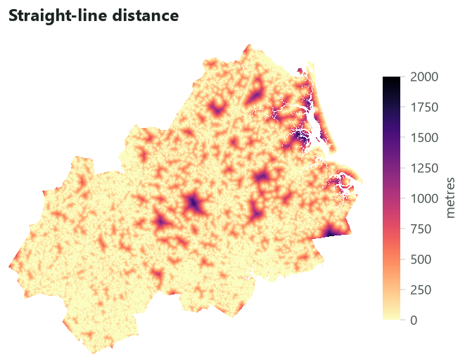
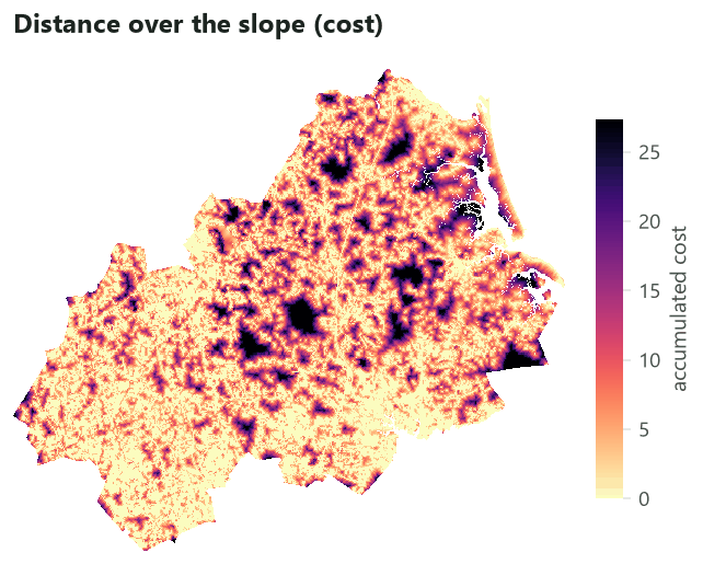
dynamic.distance_to: the distance from every cell to the nearest cell of some classes, as the exact straight-line (Euclidean) distance between cell centres, in map units or in cells. Given a cost (a transition of conductances, see grid distances), it gives instead the accumulated cost of the cheapest path, so that a steep slope or a river makes built land "farther away" than its straight-line distance.dynamic.share_of: the share of the cells in a window around each cell that hold some classes (a 3 x 3 window of ones by default, or any window of weights). This is the enrichment of Verburg et al. (2004) in its simplest form: how common built land, or forest, is in the neighbourhood.


When to use it#
Use a dynamic driver when a driver is computed from the land use that the model changes, and when the simulation is long enough for the change to matter. Typical cases:
- Urban growth: the distance to existing built land, the density of built land around a cell. Urban models have relied on such neighbourhood effects since the first cellular automata (White & Engelen, 1993).
- Agricultural frontiers: the distance to the nearest field or to the deforestation front.
- Abandonment and regrowth: the share of forest around a field, a proxy of the seed rain that lets it return to forest.
- Regional land use in CLUE-S, where neighbourhood variables are added to the location regressions (Verburg et al., 2004).
It is not needed for drivers that do not depend on land use (slope, soil, climate in a short run), nor for drivers that change for other reasons (a new road planned for 2030): those are better given as a series of maps, one per period, read inside the loop.
A dynamic driver is one way to put neighbourhood effects into a model. The alternatives are the
neighbourhood rules of CLUE-S (a class may go only where a share of its neighbours already has it; see
the rules of CLUE-S), the patch-based allocation of Dinamica EGO's
Expander or of PLUS (see PLUS and CARS), and a cellular automaton written
by hand with nbsum or nbmean in raster.calc (see
a cellular automaton by hand). A dynamic driver differs
from them in one way: its effect is estimated from the data (it has a coefficient in the regression), not set
by hand.
What you need#
- A land use map at the start and at least one later map, so that the model can be fitted on observed
change. Here: lulcc's example data of the Plum Island Ecosystems in Massachusetts (Moulds et al., 2015), a
raster of 497 x 434 cells of about 100 m with three classes, 1 Forest, 2 Built and 3 Other, mapped in 1985,
1991 and 1999 (
pie_landuse.tif, a band per year named by the year). - The drivers, a raster with a band per variable: here
pie_drivers.tifwithelevation,slopeanddist_built_1985. - A model with a regression on the land use driver. This tutorial builds a CLUE-S model as the full CLUE-S model does, with lulcc's settings that converge on this landscape.
Check the cells are square
dynamic.distance_to gives map units only for square cells. Pie's cells are 99.92 m wide and 99.95 m
high, so Terraflux refuses unit = "map" with distances in map units need square cells. Ask for the
distance in cells (unit = "cells") and multiply it by the cell's side with raster.calc, as below.
Build the model#
The model has two parts. Outside the loop, everything that is computed once: the driver at the start, the regressions, the demand, the random number generator and the history of each cell. Inside the loop, what must be computed again at every step: the driver, the stack of drivers holding it, the suitability, and the allocation.
Step 1: the driver at the start, and the regressions#
The regressions must be fitted on the same driver that the loop will compute. lulcc's dist_built_1985
was computed by its authors from their own map of built land; compared with the distance Terraflux computes from
the 1985 map, half the cells agree to the centimetre, but 10 % differ by more than 137 m and some built cells
have a distance of up to 921 m in lulcc's layer. If the regression were fitted on lulcc's layer and the loop
then gave it Terraflux's distance, the very first step would already see a different driver than the one the
coefficients were estimated on. So the model computes the driver from the start map first (nodes 1 to 3) and
fits the regressions on that.
Model file (TOML)
format = "terraflux/1"

[inputs.start]
kind = "map"
path = "pie_landuse.tif"
band = "1985"

[inputs.mid]
kind = "map"
path = "pie_landuse.tif"
band = "1991"

[inputs.drivers]
kind = "stack"
path = "pie_drivers.tif"

[[nodes]]
id = "near_built_0"
op = "dynamic.distance_to"
inputs = { landscape = "$start" }
params = { classes = 2, unit = "cells" }

[[nodes]]
id = "in_metres_0"
op = "raster.calc"
inputs = { d = "near_built_0.distance" }
params = { expression = "d * 99.92" }

[[nodes]]
id = "drivers_0"
op = "stack.set"
inputs = { stack = "$drivers", map = "in_metres_0.map" }
params = { name = "dist_built_1985" }

[[nodes]]
id = "expansion"
op = "raster.calc"
inputs = { t0 = "$start", t1 = "$mid" }
params = { expression = "None if t0 == 2 else t1" }

[[nodes]]
id = "regression"
op = "glm.fit"
inputs = { landscape = "expansion.map", drivers = "drivers_0.stack" }
params = { formulas = { 1 = ["elevation", "slope"], 2 = ["elevation", "slope", "dist_built_1985"], 3 = ["elevation", "slope"] } }
Node by node:
near_built_0(dynamic.distance_to) reads the 1985 map ($start, the model's input of that name) and gives the distance from every cell to the nearest cell of class 2, Built, in cells. In the application: find dynamic in the library, click dynamic.distance_to, and drag from themapoutput of the inputstartto itslandscapeinput; in the Node pane setclassesto 2 andunittocells.in_metres_0(raster.calc) multiplies the distance by 99.92, the side of a cell in metres, so that the driver has the units of the original layer. Its inputdis the outputdistanceof node 1.drivers_0(stack.set) takes the stack of drivers and puts the new map in the layer nameddist_built_1985, replacing lulcc's layer of that name (a name not found would be added at the end). The name is only a label: it is the name the regression's formula uses, so the coefficients will be estimated on this layer, and the loop will later put a newer map under the same label.expansion(raster.calc) makes the map the regressions learn from: no value (None) where the cell was already built in 1985, and the class of 1991 everywhere else. The reason is the most important pitfall of dynamic drivers, explained in Common pitfalls: a regression of where built land is on the distance to built land learns nothing but "built land is at distance 0 from built land".regression(glm.fit) fits a logistic regression per class on the cells that have a value inexpansion(76,441 cells, those not built in 1985), with lulcc's formulas: Forest and Other on elevation and slope, Built on elevation, slope and the distance to built land.
The fitted coefficients of Built are an intercept of -2.043, +0.0057 per metre of elevation, -0.037 per degree of slope and -0.0055 per metre of distance to built land: every 100 m farther from built land divides the odds of becoming built by about \(e^{0.55} \approx 1.7\).
Fitting on 1985 to 1991 and validating on 1999 keeps the two periods apart, as calibration and validation should be (see the validation of a simulation).
Step 2: the pieces computed once#
The demand (how many cells each class must have each year, interpolated from the observed maps), R's random number generator and the history of each cell are computed outside the loop, exactly as in the full CLUE-S model. The demand gives 14 steps, one per year from 1985 to 1999.
Step 3: the loop#
Now the loop. control.repeat runs its body, a small graph drawn inside it, once per step. Inside the
body three kinds of reference appear:
@stepis the number of the step (1, 2, ... 14);@landscapeand@historyare carried values: at step 1 they are the loop's inputs of those names ($startandhistory.history), and at every later step they are what the body gave at the end of the step before (carry = { landscape = "allocate.landscape", history = "allocate.history" }).@landscapeis therefore always the map the previous step simulated;- names without
@(regression.model,demand.demand,$drivers) are nodes and inputs outside the loop, the same at every step.
Model file (TOML)
[[nodes]]
id = "simulation"
op = "control.repeat"
inputs = { times = "demand.steps", landscape = "$start", history = "history.history" }

[nodes.body]
carry = { landscape = "allocate.landscape", history = "allocate.history" }
collect = { maps = "allocate.landscape", info = "allocate.info", distance = "in_metres.map" }

[[nodes.body.nodes]]
id = "near_built"
op = "dynamic.distance_to"
inputs = { landscape = "@landscape" }
params = { classes = 2, unit = "cells" }

[[nodes.body.nodes]]
id = "in_metres"
op = "raster.calc"
inputs = { d = "near_built.distance" }
params = { expression = "d * 99.92" }

[[nodes.body.nodes]]
id = "drivers_now"
op = "stack.set"
inputs = { stack = "$drivers", map = "in_metres.map" }
params = { name = "dist_built_1985" }

[[nodes.body.nodes]]
id = "suitability"
op = "glm.predict"
inputs = { model = "regression.model", drivers = "drivers_now.stack", landscape = "@landscape" }

[[nodes.body.nodes]]
id = "allocate"
op = "lulcc.step"
inputs = { landscape = "@landscape", history = "@history", suitability = "suitability.suitability", demand = "demand.demand", step = "@step", rng = "rng.rng" }
params = { allocation = { method = "clue", jitter = 0.0002, scale = 0.000001, max_iter = 1000, max_diff = 50, mean_diff = 50 }, elasticity = [0.2, 0.2, 0.2] }
The whole model, ready to run
Model file (TOML)
format = "terraflux/1"

[inputs.observed]
kind = "stack"
path = "pie_landuse.tif"

[inputs.start]
kind = "map"
path = "pie_landuse.tif"
band = "1985"

[inputs.mid]
kind = "map"
path = "pie_landuse.tif"
band = "1991"

[inputs.drivers]
kind = "stack"
path = "pie_drivers.tif"

[inputs.seed]
kind = "value"
value = 1

[[nodes]]
id = "near_built_0"
op = "dynamic.distance_to"
inputs = { landscape = "$start" }
params = { classes = 2, unit = "cells" }

[[nodes]]
id = "in_metres_0"
op = "raster.calc"
inputs = { d = "near_built_0.distance" }
params = { expression = "d * 99.92" }

[[nodes]]
id = "drivers_0"
op = "stack.set"
inputs = { stack = "$drivers", map = "in_metres_0.map" }
params = { name = "dist_built_1985" }

[[nodes]]
id = "expansion"
op = "raster.calc"
inputs = { t0 = "$start", t1 = "$mid" }
params = { expression = "None if t0 == 2 else t1" }

[[nodes]]
id = "regression"
op = "glm.fit"
inputs = { landscape = "expansion.map", drivers = "drivers_0.stack" }
params = { formulas = { 1 = ["elevation", "slope"], 2 = ["elevation", "slope", "dist_built_1985"], 3 = ["elevation", "slope"] } }

[[nodes]]
id = "demand"
op = "demand.from_maps"
inputs = { maps = "$observed" }
params = { times = [0, 6, 14] }

[[nodes]]
id = "rng"
op = "rng.r"
inputs = { seed = "$seed" }

[[nodes]]
id = "history"
op = "lulcc.history"
inputs = { landscape = "$start" }

[[nodes]]
id = "simulation"
op = "control.repeat"
inputs = { times = "demand.steps", landscape = "$start", history = "history.history" }

[nodes.body]
carry = { landscape = "allocate.landscape", history = "allocate.history" }
collect = { maps = "allocate.landscape", info = "allocate.info", distance = "in_metres.map" }

[[nodes.body.nodes]]
id = "near_built"
op = "dynamic.distance_to"
inputs = { landscape = "@landscape" }
params = { classes = 2, unit = "cells" }

[[nodes.body.nodes]]
id = "in_metres"
op = "raster.calc"
inputs = { d = "near_built.distance" }
params = { expression = "d * 99.92" }

[[nodes.body.nodes]]
id = "drivers_now"
op = "stack.set"
inputs = { stack = "$drivers", map = "in_metres.map" }
params = { name = "dist_built_1985" }

[[nodes.body.nodes]]
id = "suitability"
op = "glm.predict"
inputs = { model = "regression.model", drivers = "drivers_now.stack", landscape = "@landscape" }

[[nodes.body.nodes]]
id = "allocate"
op = "lulcc.step"
inputs = { landscape = "@landscape", history = "@history", suitability = "suitability.suitability", demand = "demand.demand", step = "@step", rng = "rng.rng" }
params = { allocation = { method = "clue", jitter = 0.0002, scale = 0.000001, max_iter = 1000, max_diff = 50, mean_diff = 50 }, elasticity = [0.2, 0.2, 0.2] }

[outputs.maps]
from = "simulation.maps"

[outputs.steps]
from = "simulation.info"

[outputs.distance]
from = "simulation.distance"
The body, in the order its nodes run at every step:
near_built(dynamic.distance_to) computes the distance to built land from@landscape. At step 1 that is the map of 1985, so it gives the same map asnear_built_0; at step 2 it is the map step 1 simulated, with its new houses; and so on.in_metresconverts it to metres, as outside the loop.drivers_now(stack.set) puts it into$drivers, the original stack, under the namedist_built_1985. It starts again from the original stack at every step rather than from the previous step's stack: only one layer changes, so either would work, but reading the input keeps the step independent of the one before.suitability(glm.predict) applies the coefficients ofregression.modelto the drivers of this step. This node must be inside the body: a node outside the loop runs once, before the first step, and could never see a driver computed inside it. Itslandscapeinput (@landscape) only marks the cells without a value, which stay without one.allocate(lulcc.step) allocates the step's demand with CLUE-S, on the new suitability.
At the end of the step, carry passes allocate.landscape and allocate.history on as the next
@landscape and @history. collect keeps a series of values, one per step: maps (the simulated maps,
written as a raster of 14 bands), info (the allocation's iterations and the cells of each class, a table) and
distance (the driver each step saw, useful to check it moves). After the last step, simulation.landscape
is the final map and simulation.maps the series.
In the application
Double-click the simulation node (or Open inside in the Node pane) to open the body. Its left
column lists what the body can read: @step, @landscape, @history, the model's inputs and the outer
nodes. Add the four new nodes from the library, connect @landscape to near_built's landscape, and
connect drivers_now.stack to suitability's drivers. In the Node pane of the simulation node, add
distance = in_metres.map to its collected outputs. The trail at the top of the canvas takes you back to the
whole model.
The static model differs only in where the suitability is computed: a glm.predict outside the loop, on
drivers_0.stack, read by allocate at every step.
The static model, for comparison
Model file (TOML)
format = "terraflux/1"

[inputs.observed]
kind = "stack"
path = "pie_landuse.tif"

[inputs.start]
kind = "map"
path = "pie_landuse.tif"
band = "1985"

[inputs.mid]
kind = "map"
path = "pie_landuse.tif"
band = "1991"

[inputs.drivers]
kind = "stack"
path = "pie_drivers.tif"

[[nodes]]
id = "near_built_0"
op = "dynamic.distance_to"
inputs = { landscape = "$start" }
params = { classes = 2, unit = "cells" }

[[nodes]]
id = "in_metres_0"
op = "raster.calc"
inputs = { d = "near_built_0.distance" }
params = { expression = "d * 99.92" }

[[nodes]]
id = "drivers_0"
op = "stack.set"
inputs = { stack = "$drivers", map = "in_metres_0.map" }
params = { name = "dist_built_1985" }

[[nodes]]
id = "expansion"
op = "raster.calc"
inputs = { t0 = "$start", t1 = "$mid" }
params = { expression = "None if t0 == 2 else t1" }

[[nodes]]
id = "regression"
op = "glm.fit"
inputs = { landscape = "expansion.map", drivers = "drivers_0.stack" }
params = { formulas = { 1 = ["elevation", "slope"], 2 = ["elevation", "slope", "dist_built_1985"], 3 = ["elevation", "slope"] } }

[[nodes]]
id = "suitability"
op = "glm.predict"
inputs = { model = "regression.model", drivers = "drivers_0.stack", landscape = "$start" }

[[nodes]]
id = "demand"
op = "demand.from_maps"
inputs = { maps = "$observed" }
params = { times = [0, 6, 14] }

[[nodes]]
id = "rng"
op = "rng.r"
inputs = { seed = 1 }

[[nodes]]
id = "history"
op = "lulcc.history"
inputs = { landscape = "$start" }

[[nodes]]
id = "simulation"
op = "control.repeat"
inputs = { times = "demand.steps", landscape = "$start", history = "history.history" }

[nodes.body]
carry = { landscape = "allocate.landscape", history = "allocate.history" }
collect = { maps = "allocate.landscape" }

[[nodes.body.nodes]]
id = "allocate"
op = "lulcc.step"
inputs = { landscape = "@landscape", history = "@history", suitability = "suitability.suitability", demand = "demand.demand", step = "@step", rng = "rng.rng" }
params = { allocation = { method = "clue", jitter = 0.0002, scale = 0.000001, max_iter = 1000, max_diff = 50, mean_diff = 50 }, elasticity = [0.2, 0.2, 0.2] }
Run it#
Run the model with Ctrl+Enter on the simulation node, or from the command line, in the folder that holds
the two rasters:
terraflux check dynamic.toml
terraflux run dynamic.toml --out dynamic     # writes dynamic/maps.tif, steps.csv, distance.tif
On a laptop each run takes about 20 seconds: computing a distance over 216,000 cells and predicting three regressions at each of 14 steps adds little to the allocation itself. Every step converged (the demand met to within 50 cells), so the two runs have exactly the same amount of built land each year; they differ only in where it went.
Read the results#
The growth, year by year#
The slider shows the dynamic run. Built land of 1985 is grey, land built in earlier steps pink, and the land built in the step shown dark red. The numbers beside it come from the run: the share of the map that is built, how many new built cells lie more than 500 m from any built land of 1985 ("built > 500 m away"), and the mean of the distance driver over the map at the start of the step ("mean distance").


For five steps the two runs are almost the same. Then the dynamic run starts building far from the built land of 1985: by 1999 it has placed 355 cells more than 500 m away, the static run 133. The reason is the feedback. CLUE-S scatters some change onto cells of middling suitability (its allocation competes classes cell by cell, with a small random jitter). In the static run, a house built far away changes nothing. In the dynamic run, it makes the cells around it nearer to built land, hence more suitable for built land at the next step, and the next houses gather around it: outposts grow into small clusters, which seed further growth.
The final maps#


The maps look alike at this scale: in both, new built land is scattered in small groups through the existing suburbs. The difference is in the tail, which the chart below measures: where new built land went, by its distance to the built land of 1985.
Half of the land actually built between 1985 and 1999 lies within 100 m of the built land of 1985, and only 1.4 % lies more than 500 m away. The static run puts 57.6 % within 100 m (too close) and 2.0 % beyond 500 m; the dynamic run puts 47.3 % within 100 m (nearer the observed 49.5 %) but 5.3 % beyond 500 m, almost four times the observed share. The feedback moved the model's growth outwards, partly in the right direction and partly too far.
Does it agree better with 1999?#
The figure of merit (Pontius et al., 2008) measures the agreement on change: the cells that the model changed
correctly, divided by all the cells that changed in the observed map or in the simulated one. It is 0 for no
agreement and 1 for a perfect simulation. Comparing the maps in blocks of 2, 4, 8 and 16 cells forgives errors
of location smaller than a block (Pontius et al., 2011). Both values come from validate.three_map run on
the final maps.
| Blocks of | 1 cell | 2 cells | 4 cells | 8 cells | 16 cells |
|---|---|---|---|---|---|
| Static driver, all classes | 0.056 | 0.073 | 0.107 | 0.155 | 0.196 |
| Dynamic driver, all classes | 0.053 | 0.070 | 0.101 | 0.147 | 0.188 |
| Static driver, Built | 0.023 | 0.032 | 0.052 | 0.067 | 0.043 |
| Dynamic driver, Built | 0.023 | 0.032 | 0.052 | 0.066 | 0.043 |
The two runs are equally poor at the level of the cell, and the dynamic one is slightly worse at every resolution. Figures of merit below 0.1 at the resolution of the data are common for land change models (Pontius et al., 2008), and this one uses only three drivers. The lesson is not that dynamic drivers are useless, but that on Plum Island, from 1985 to 1999, growth stayed next to the existing suburbs more than the feedback assumes. A dynamic driver is a hypothesis about a process (new houses attract houses), and the comparison with an observed map is its test.
In the literature
Neighbourhood variables recomputed during the simulation are standard in CLUE-S applications to urban and peri-urban change (Verburg et al., 2004) and in the land use cellular automata descended from White and Engelen (1993). Report which drivers were dynamic, how they were computed (distance or share, window, classes) and the agreement of the model with and without them on a period not used for fitting.
How to report it#
Give the formula of each regression and its coefficients (the glm output of the model holds them), say which
drivers were recomputed at each step and how, give the period of calibration and the period of validation, and
report the figure of merit at several resolutions for the model with and without the dynamic driver, with a
null model of no change for reference.
Settings that change the answer#
- The window of
dynamic.share_of. A 3 x 3 window measures the immediate neighbours (a house next door); a 9 x 9 window, about 900 m across here, measures the character of the area (a suburb). The two figures at the top of this page show how different the two drivers are on the same map. The regression must be fitted with the same window as the loop uses. - Distance or cost. A cost distance makes the driver respect barriers (rivers, steep slopes, a motorway with few crossings). Use it when the barrier is real for the process: people commute along roads, not across marshes.
- The classes.
classes = 2measures the distance to built land;classes = [2, 3]would count built and other land together. Each choice is a different hypothesis. - What the regression is fitted on. Presence or expansion (below) changes the coefficient of a land use driver by orders of magnitude.
Common pitfalls#
Fitting a land use driver on where the land use is. A regression of the presence of built land on the
distance to built land is circular: every built cell has a distance of 0 and no other cell does. Fitted that
way on Pie (with landscape = "$start" in glm.fit), the regression of Built has an intercept of 24.0, a
coefficient of -0.47 per metre and explains 100 % of the deviance: a suitability of almost exactly 1 on built
cells and almost exactly 0 one cell away. The allocation then has no information about where to put new built
land (every non-built cell has the same suitability, about zero) and scatters it by chance. Fit land use
drivers on where the class appeared in an observed period (the expansion map above), as the land
expansion analysis of PLUS does (see PLUS and CARS).
A driver the loop computes differently from the one the regression saw. If the regression is fitted on a
layer made by another program and the loop recomputes it with Terraflux, the coefficients are applied to a
different variable from step 1. Compute the starting value with the same nodes as the loop (step 1 above), and
check: the first band of the collected distance must equal the layer the regression was fitted on.
The prediction outside the loop. A glm.predict outside the body runs once and never sees the new
driver: the model is static whatever happens inside. The suitability, and everything between the driver and
it, belongs inside the body.
Wrong units. A regression fitted on metres and given cells (or the reverse) multiplies the effect of the
driver by 100. On Pie's cells, which are not exactly square, unit = "map" is refused; use cells and convert.
The edge of the map. A distance near the edge of the study area ignores built land just outside it. Compute the starting driver on a map larger than the study area when you can, or keep a buffer.
Going further#
- The next part, agents, puts decision makers into the loop: values carried from step to step like the map.
- The rules of CLUE-S shows the neighbourhood rules, a simpler way to make a class grow next to itself.
- The full CLUE-S model explains the demand, the history and the allocation used here.
- A demand per region and choosing a model compare the other models that take dynamic drivers in the same way (CARS, MOLUSCE).
- The operators:
dynamic.distance_to,dynamic.share_of,stack.set,glm.predict,cost.transition.
References#
- Moulds, S., Buytaert, W., & Mijic, A. (2015). An open and extensible framework for spatially explicit land use change modelling: the lulcc R package. Geoscientific Model Development, 8(10), 3215–3229. https://doi.org/10.5194/gmd-8-3215-2015
- Pontius, R. G., Jr., Boersma, W., Castella, J.-C., Clarke, K., de Nijs, T., Dietzel, C., et al. (2008). Comparing the input, output, and validation maps for several models of land change. The Annals of Regional Science, 42(1), 11–37. https://doi.org/10.1007/s00168-007-0138-2
- Pontius, R. G., Jr., Peethambaram, S., & Castella, J.-C. (2011). Comparison of three maps at multiple resolutions: a case study of land change simulation in Cho Don District, Vietnam. Annals of the Association of American Geographers, 101(1), 45–62. https://doi.org/10.1080/00045608.2010.517742
- Verburg, P. H., de Nijs, T. C. M., Ritsema van Eck, J., Visser, H., & de Jong, K. (2004). A method to analyse neighbourhood characteristics of land use patterns. Computers, Environment and Urban Systems, 28(6), 667–690. https://doi.org/10.1016/j.compenvurbsys.2003.07.001
- Verburg, P. H., Soepboer, W., Veldkamp, A., Limpiada, R., Espaldon, V., & Mastura, S. S. A. (2002). Modeling the spatial dynamics of regional land use: the CLUE-S model. Environmental Management, 30(3), 391–405. https://doi.org/10.1007/s00267-002-2630-x
- White, R., & Engelen, G. (1993). Cellular automata and fractal urban form: a cellular modelling approach to the evolution of urban land-use patterns. Environment and Planning A, 25(8), 1175–1199. https://doi.org/10.1068/a251175