Connectivity as a graph

This series is about one question: how well are the pieces of a habitat connected for a species that has to move between them? In this first part you turn a land cover map into a graph, the object that all of the series is built on: every forest patch becomes a point (a node), and every pair of patches close enough for an animal to cross the gap between them is joined by a line (a link). You build it in Terraflux from a real map of the countryside around Hannover in Germany, count its links and its groups of connected patches for species that cross 250 m to 10 km of open land, and learn the words and the choices the rest of the series relies on. At the end you will have a model that reads any land cover map and gives its habitat graph, ready for the connectivity indices of part 2.

The idea#

Structural and functional connectivity#

Ecologists started talking about landscape connectivity in the 1980s and 1990s, when it became clear that the amount of habitat is not the whole story: two landscapes with the same area of forest can be very different places for a forest bird, depending on whether the forest is one block, a few large blocks close together, or a dust of small woods scattered in fields. Taylor et al. (1993) gave the definition most studies still quote: connectivity is "the degree to which the landscape facilitates or impedes movement among resource patches".

Two words in that definition matter. Facilitates or impedes means connectivity is a property of the landscape for a given movement, not of the map alone. Among resource patches means it is about getting from one patch of habitat to another. Tischendorf and Fahrig (2000) made the distinction that runs through this series:

• Structural connectivity describes the map only: how close the patches are, how many corridors join them. It ignores the species.
• Functional connectivity describes how a particular species moves through that structure: the same gap of 800 m of wheat is a wall for a ground beetle and a short walk for a pine marten.

Enlarge

Every method in this series is a way of putting a species into a map: a dispersal distance, a probability of crossing, a resistance of the land between patches. That is what makes the results functional, and it is also where most of the uncertainty lies.

A landscape as a graph#

Urban and Keitt (2001) proposed to describe habitat with the mathematics of networks, graph theory: a graph is a set of nodes and a set of links between pairs of them, and decades of work on graphs give ready answers to questions such as "which nodes can reach which?", "how many steps between two nodes?" or "which node, if removed, would cut the network in two?". In a landscape graph (or habitat graph):

• a node is a patch of habitat, with an attribute, usually its area (the habitat it offers);
• a link joins two patches that a disperser can move between directly, and may carry a distance or a probability of moving.

Minor and Urban (2008) showed how far this goes for conservation planning: the graph of a region tells which patches hold the network together, which groups of patches are isolated from the rest, and where adding a patch would join two groups. Galpern et al. (2011) review how such graphs are built and used. Its great advantage is economy: a map of 250,000 cells becomes a graph of 154 nodes, and questions about the whole landscape become fast to answer.

How far apart are two patches?#

The distance between two patches can be measured in three ways, and the choice matters:

• Between centroids (the centre of each patch): simple and fast, but two large patches that touch along an edge can be kilometres apart centre to centre.
• Between edges (the gap between their nearest cells): the distance an animal actually has to cross. This is what Conefor and most studies of forest patches use, and what this series uses.
• Least-cost (the cheapest route through a map of resistance): the distance weighted by how hard the land along it is to cross, from the centroid of one patch to the centroid of the other (as Makurhini measures it). It is the subject of part 4.

Links with probabilities#

A threshold says a disperser crosses 999 m and never 1,001 m. Real dispersal fades: most individuals settle close to where they were born and a few go far. The usual model is a negative exponential kernel, in which the probability of moving between two patches falls with the distance between them. Choose the distance \(d\) at which the probability is \(p\) (half of the dispersers, say, cross 1 km); then at any other distance

The threshold graph of this part and the kernel of part 2 are two views of the same graph: Terraflux's habitat graph stores the distances, and every operator that reads it takes the distance (and, for probabilities, the probability at that distance) as a setting. One graph serves every species.

When to use it#

A habitat graph is the right tool when your question is about patches and the moves between them:

• Which patches form a connected group for a species, and how many isolated groups the habitat falls into. Keitt et al. (1997) used the components of the graph of Mexican spotted owl habitat to find the dispersal distance at which the landscape "percolates" from many groups into one.
• How connected a whole landscape is, and how that changes over time or between plans: the indices of part 2, used for example to follow the connectivity of European forests between 1990 and 2000 (Saura et al., 2011).
• Which patches and links matter most, to protect or to restore: part 3.
• How well a network of reserves is connected: ProtConn, part 6.

What it is not for: where in the matrix animals move (the exact route between two patches) is better answered by least-cost paths (grid distances) or circuit theory (circuit connectivity). The shape of the habitat (cores, edges, corridors) is the subject of MSPA (habitat patterns), which this series turns into a graph in part 5.

What you need#

• A map of the habitat, or a land cover map whose classes you can name as habitat. Here, clc_100m.tif (29 KB): CORINE Land Cover for a square of 50 × 50 km north-west of Hannover, Germany, around Lake Steinhude, in the European equal-area projection (EPSG:3035), with cells of 100 m. It was made from CORINE's map at 25 m (clc.tif, 290 KB, the map of the MSPA tutorial) by raster.resample with resampling = "mode": each 100 m cell takes the most common class of its sixteen 25 m cells. Its forests are CORINE's classes 23 (broad-leaved), 24 (coniferous) and 25 (mixed).
• A coordinate system in metres with square cells. Distances and areas are computed from the cells, so a map in degrees gives wrong numbers (see the pitfalls).
• One or more dispersal distances for your species: from tracking or genetic studies, from reviews (for birds and mammals, natal dispersal scales with body size and home range, Sutherland et al., 2000), or, when little is known, a range that brackets the plausible values.

The application's template Habitat network (Conefor) (Templates > Connectivity) builds the graph and the indices of part 2 on a landscape drawn by chance; replace its first node with a raster.read of your map.

Enlarge

Build the model#

1. Read the map#

Add raster.read (library, subject Data preparation, or press / and type read) and choose clc_100m.tif in its path. Its output map is the land cover, one class per cell.

2. Build the habitat graph#

Add conn.graph_from_raster (library, subject Habitat networks) and drag from land.raster to its input map. This one node does three things: it finds the patches of habitat (groups of habitat cells that touch, including at a corner: directions = 8), measures the attribute of each (its area), and measures the distance between every pair of patches. Its output graph is a habitat graph, a value that only the operators of the subject Habitat networks read.

The settings that matter:

• habitat = [23, 24, 25]: the classes that are habitat. Every other class is the matrix the species has to cross. A map that is already a patch map (a patch number in each cell) needs no habitat.
• area_unit = "ha": the patches' areas in hectares. The units do not change any index of the series, but they make the tables readable.
• distance = "edge": the gap between the closest cells of two patches, in metres. centroid (the default) is the distance between their centres; least-cost and commute-time use a resistance map, between the centroids (part 4).
• landscape_area = 250000: the area of the whole study area in hectares (500 × 500 cells of 1 ha). The indices of part 2 divide by it; it does not change the graph.

format = "terraflux/1"

[[nodes]]
id = "land"
op = "raster.read"
params = { path = "clc_100m.tif" }
note = "CORINE Land Cover, cells of 100 m."

[[nodes]]
id = "graph"
op = "conn.graph_from_raster"
inputs = { map = "land.raster" }
params = { habitat = [23, 24, 25], area_unit = "ha", distance = "edge", landscape_area = 250000 }
note = "The forest patches, their areas (ha) and the gaps between their edges (m)."

3. Count links and components#

Add conn.overall and connect graph.graph to its graph. It describes the whole graph, one row per distance: set distance = [250, 500, 1000, 2000, 5000, 10000] (metres, because the graph's distances are in metres) and metrics = ["A", "NC", "NL", "H"]. A is the total habitat area, NC the number of components, NL the number of links (pairs no farther apart than the distance) and H the Harary index, a sum over all pairs of \(1 / (\text{steps between them})\). Without metrics, it also computes the indices of part 2.

4. Map the components#

conn.components gives, for one distance, the component of every patch: a table of id and component. A table of patches becomes a map with conn.to_map: it takes the graph (to know which cells make each patch) and the table, and paints every patch with the value of its row in column.

format = "terraflux/1"

[[nodes]]
id = "land"
op = "raster.read"
params = { path = "clc_100m.tif" }
note = "CORINE Land Cover, cells of 100 m."

[[nodes]]
id = "graph"
op = "conn.graph_from_raster"
inputs = { map = "land.raster" }
params = { habitat = [23, 24, 25], area_unit = "ha", distance = "edge", landscape_area = 250000 }
note = "The forest patches, their areas (ha) and the gaps between their edges (m)."

[[nodes]]
id = "overall"
op = "conn.overall"
inputs = { graph = "graph.graph" }
params = { distance = [250, 500, 1000, 2000, 5000, 10000], metrics = ["A", "NC", "NL", "H"] }
note = "A row per distance: habitat area, components, links, Harary."

[[nodes]]
id = "components"
op = "conn.components"
inputs = { graph = "graph.graph" }
params = { distance = 2000 }
note = "The component of every patch for a species that crosses 2 km."

[[nodes]]
id = "component_map"
op = "conn.to_map"
inputs = { graph = "graph.graph", table = "components.table" }
params = { column = "component" }
note = "Each patch painted with its component."

[[plots]]
id = "plot"
title = "Components at 2 km"
layers = [{ from = "component_map.map" }]

terraflux run graph.toml

Read the results#

The patches#

The forest falls into 154 patches covering 51,569 ha. They are very unequal: the five largest (9,151, 7,071, 4,599, 2,884 and 2,860 ha) hold almost half of the forest, while the median patch is 57 ha. This is typical of agricultural landscapes in Europe, and it is the first thing to look at, because every index of the series weighs patches by their area.

Enlarge

The links at 1 km#

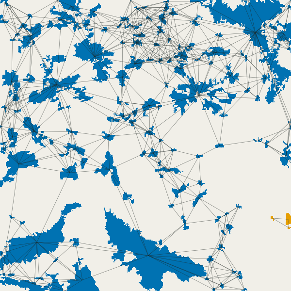
For a species that crosses up to 1 km of open land, 120 pairs of patches are linked. Drawn between the patches' centres, they show the structure of the graph at once: dense clusters of woods in the north and the north-west, chains along the valleys, and many patches with no link at all.

Enlarge

Components at increasing distances#

Move the slider: each frame is the components of the graph at one distance, each component in its own colour (grey: patches alone), with the links drawn.

Enlarge

PlayDispersal distance

How to read these numbers:

• The fall of NC tells the critical distance. The number of components does not fall evenly: it drops from 56 to 11 between 1 and 2 km, as the woods of the north-west and the north join the large north-eastern forest. Keitt et al. (1997) called such a jump a critical scale: species that cross less than it live in a fragmented landscape, species that cross more in a connected one. For conservation it is the range where small changes (one wood lost, one restored) change the most.
• NL grows faster than connectivity. Links multiply with distance (1,690 at 10 km), but most new links join patches that were already connected through others. That redundancy is why NL alone is a poor index: it does not say whether the links matter.
• The large southern forest stays apart longest. At 2 km it is still its own component with a few neighbours; only at 5 km does it join the rest. For a species of the south, the map is two landscapes.

Settings that change the answer#

• The dispersal distance. It changes everything, as the slider shows. When the distance of your species is uncertain, run several (the distance of conn.overall takes a list) and report the range.
• Edge or centroid distances. With distance = "centroid" the same pairs are farther apart (by about half the size of each patch), so fewer are linked at any threshold, and large patches lose the most. Use edges for areas of habitat and centroids only for small patches or points (ponds, nest sites).
• 4 or 8 neighbours. With directions = 4, cells that touch only at a corner are separate patches, so a diagonal chain of cells becomes several patches. With 100 m cells the difference is small; on fine maps (rows of trees at 10 m) it can be large.
• The cell size. Resampling from 25 m to 100 m merges woods that were a few metres apart and drops woods smaller than half a cell; the "mode" resampling also makes thin forest strips vanish. Build the graph at the finest resolution the analysis can afford, and never compare graphs made from maps of different resolution.
• The habitat classes. Adding CORINE's class 29 (transitional woodland-shrub) to the habitat joins many patches. The habitat definition is an ecological choice: state it, and test the alternatives.

Common pitfalls#

• A map in degrees. Areas and distances come from the cells, so cells must be in metres and square. Reproject first (raster.reproject, with resampling = "near" for classes).
• No-data around the map. The study area's border cuts patches in two and hides the patches just outside it, so patches near the border look smaller and more isolated than they are. Analyse a larger area than you report, or keep a buffer of the dispersal distance around it.
• Threshold distance in the wrong unit. The graph's distances are in distance_unit (metres by default); a distance = 2 meant as kilometres links almost nothing.
• Patches that are "one" for you but two for the map. A road of one cell splits a forest into two patches at distance 100 m. That may be right (for a beetle) or wrong (for a deer): decide whether roads belong to the habitat or the matrix before building the graph.
• Too many patches. The number of pairs grows with the square of the number of patches: 154 patches make 11,781 pairs, 10,000 patches 50 million. For very large maps, drop the smallest patches (paint every patch with its area by conn.nodes and conn.to_map, then keep the large ones with raster.calc) or set max_distance so that only nearby pairs are kept.

Going further#

• Part 2: IIC, PC and the equivalent connected area: one number for the connectivity of the whole graph, and how it changes with the dispersal distance.
• Part 3: the importance of each patch.
• Part 4: least-cost links: distances through a map of resistance instead of straight gaps.
• Habitat patterns: the shapes of the habitat, before the graph.
• The operators: conn.graph_from_raster, conn.overall, conn.components, conn.to_map, conn.nodes, conn.distances, conn.graph, conn.write_conefor.

References#

• Galpern, P., Manseau, M., & Fall, A. (2011). Patch-based graphs of landscape connectivity: a guide to construction, analysis and application for conservation. Biological Conservation, 144(1), 44–55. https://doi.org/10.1016/j.biocon.2010.09.002
• Keitt, T. H., Urban, D. L., & Milne, B. T. (1997). Detecting critical scales in fragmented landscapes. Conservation Ecology, 1(1), 4. https://doi.org/10.5751/ES-00015-010104
• Minor, E. S., & Urban, D. L. (2008). A graph-theory framework for evaluating landscape connectivity and conservation planning. Conservation Biology, 22(2), 297–307. https://doi.org/10.1111/j.1523-1739.2007.00871.x
• Saura, S., Estreguil, C., Mouton, C., & Rodríguez-Freire, M. (2011). Network analysis to assess landscape connectivity trends: application to European forests (1990–2000). Ecological Indicators, 11(2), 407–416. https://doi.org/10.1016/j.ecolind.2010.06.011
• Sutherland, G. D., Harestad, A. S., Price, K., & Lertzman, K. P. (2000). Scaling of natal dispersal distances in terrestrial birds and mammals. Conservation Ecology, 4(1), 16. https://doi.org/10.5751/ES-00184-040116
• Taylor, P. D., Fahrig, L., Henein, K., & Merriam, G. (1993). Connectivity is a vital element of landscape structure. Oikos, 68(3), 571–573. https://doi.org/10.2307/3544927
• Tischendorf, L., & Fahrig, L. (2000). On the usage and measurement of landscape connectivity. Oikos, 90(1), 7–19. https://doi.org/10.1034/j.1600-0706.2000.900102.x
• Urban, D., & Keitt, T. (2001). Landscape connectivity: a graph-theoretic perspective. Ecology, 82(5), 1205–1218. https://doi.org/10.1890/0012-9658(2001)082[1205:LCAGTP]2.0.CO;2