

Continuous surfaces, part 2 of 4
Surface metrics: texture without patches
Describe a continuous map, such as greenness, canopy height or elevation, by its roughness, the shape of its distribution and its spatial structure, without cutting it into patches first.
- Level
- Intermediate
- Time
- 45 min
In this tutorial you describe the greenness of a forested landscape in Oregon without ever drawing a patch. You will see first why cutting a continuous map into "forest" and "non-forest" can change the answer more than the landscape does; then remove the broad trend of the map, measure what remains with the surface metrics of the ISO 25178 standard (its roughness, the shape of its distribution, its slopes, its peaks and its spatial structure), read its bearing area curve, and map its texture in moving windows. At the end you will know which surface metrics to compute, how to read them, how to report them, and which settings change them.
The idea#
Most of landscape ecology, and most of Terraflux's tutorials, look at landscapes as maps of classes: forest or pasture, habitat or not, each patch (a group of touching cells of the same class) with a sharp edge. This is the patch-mosaic model, on which landscape metrics such as FRAGSTATS' rest (see Landscape metrics). It fits landscapes shaped by people: a field ends at a fence.
Many variables that matter to organisms do not have edges: canopy height, greenness, soil moisture, temperature, elevation. A forest thinning into woodland has no line to draw, and a bird does not switch from "forest" to "non-forest" at 60 % canopy cover. McGarigal & Cushman (2005) called the alternative the gradient model of landscape structure: structure as continuous variation in space, of which patches are only a special case.
The trouble with patches on a continuous map is the threshold. To count forest patches on a map of
greenness, you must decide what greenness makes a forest, and that number rarely comes from the ecology. Move the
slider to see what the choice does on the map of this tutorial. The map is a composite of summer greenness
(NDVI, see below) at 30 m; every frame is the same map, cut at a different value, and measured with
metrics.class:


Each frame comes from a model like this one, with the threshold in the expression:
Model file (TOML)
format = "terraflux/1"

[[nodes]]
id = "ndvi"
op = "raster.read"
params = { path = "ndvi.tif" }

[[nodes]]
id = "habitat"
op = "raster.calc"
inputs = { n = "ndvi.raster" }
params = { expression = "2 if n >= 0.7 else 1" }
note = "Forest where NDVI is 0.7 or more."

[[nodes]]
id = "metrics"
op = "metrics.class"
inputs = { map = "habitat.map" }
params = { metrics = ["pland", "np"], show = "pland" }
note = "Share of the map and number of patches of each class."
At 0.60 the "forest" is one nearly continuous cover with 21 holes in it; at 0.70 it is 814 fragments. Nothing in the landscape changed between the two; only the definition did. A study that reported "814 forest patches" would be reporting its threshold as much as its forest. The thresholds that change the answer most are those in the middle of the distribution of values, where most cells are.
Surface metrics describe the continuous map as it is. They come from engineering, where the texture of machined and polished surfaces (a cylinder's bore, a sheet of paper) has long been measured as the deviations of heights from a reference plane; the areal (two-dimensional) parameters are standardised as ISO 25178. McGarigal et al. (2009) proposed them to landscape ecologists as an alternative to patch metrics, with the "height" of the surface being any continuous variable: greenness, canopy height, a habitat suitability, the elevation itself. Kedron et al. (2018) compared how they behave on landscape models across ecoregions and scales, and Smith et al. (2021) made them available in the R package geodiv, which Terraflux reproduces through landschaft's C++ (the same values, with geodiv's known errors corrected).
The metrics fall into families. The first two need only the list of heights; the others need their positions.
Key idea: amplitude, the size of the variation
With \( z_i \) the height (here, the greenness) of cell \( i \), \( \bar z \) the mean height and \( N \) the number of cells with a value:
\( S_a \), the average roughness, is the mean distance of the cells from the mean; \( S_q \), the root mean square roughness, is the standard deviation of the heights, which weights large deviations more. Both are in the units of the variable.
Key idea: the shape of the distribution
The skewness \( S_{sk} \) is negative when most cells sit a little above the mean and a few lie far below it (a high plateau cut by deep valleys: a closed canopy with clearings), positive in the opposite case (a plain with scattered peaks: lone trees in a grassland). The excess kurtosis \( S_{ku} \) is 0 for a normal distribution and large when a few extreme cells make long tails. (Terraflux's \( S_{sk} \) is geodiv's adjusted skewness, corrected for small samples.)
Two surfaces can have the same amplitude and distribution and look nothing alike: one with heights in fine speckles, another in broad waves. Spatial metrics see the difference. The central tool is the areal autocorrelation function (\( \text{ACF} \)): how similar the surface is to a copy of itself shifted by a lag, 1 at no shift, falling as the shift grows.
Key idea: autocorrelation length
\( S_{al} \), the autocorrelation length, is the shortest distance at which the autocorrelation function falls to 0.2: beyond it, the surface is nearly unrelated to itself. It is the size of the grain of the texture, in map units (metres). \( S_{td} \), the texture direction, is the angle in which the texture is stretched; \( S_{rw} \), the dominant wavelength, the spacing of a repeated pattern such as ridges or rows.
Between the families sit the hybrid metrics, which combine heights and positions: \( S_{dq} \), the root mean square slope (the change of height from a cell to its neighbours) and \( S_{dr} \), how much larger the surface is than its flat footprint; the feature metrics: \( S_{ds} \), the density of summits (cells higher than their eight neighbours), and \( S_{10z} \), the mean of the five highest peaks and the five deepest valleys; and the bearing area curve, explained under the results.
When to use it#
Use surface metrics when your variable is continuous and you have no good reason to cut it:
- Vegetation structure: the heterogeneity of greenness, canopy height (from lidar) or tree cover, as a covariate of species distributions, of bird or insect diversity, of habitat quality.
- Comparing landscapes or dates without choosing one threshold for all of them: the same metric computed on every landscape, or on the same landscape before and after a disturbance.
- Texture maps: the metrics in a moving window around every cell, a map of heterogeneity at a chosen scale that enters a model like any other variable.
- Terrain: the elevation is a surface too; its surface metrics summarise a whole relief in a few numbers (for the indices of each cell, see Terrain from an elevation model).
What they are not for: when the classes are real (a road, a reservoir, a field), patch metrics describe them better and in units people understand. Surface metrics also say nothing about what lies between two places for an organism moving across them: for that, see Habitat networks and Circuit connectivity.
What you need#
- A continuous raster: one value per cell, no classes. Here
orforest.tif, a composite of summer NDVI over a forested area of south-western Oregon (its band is namedsummer_ndvi_p45_r30_2000_2016_30m), 371 × 371 cells of 1 arc-second (about 30 m), in longitude and latitude. NDVI, the normalised difference vegetation index, compares the red and near-infrared light a satellite measures; from about 0.1 for bare ground to about 0.9 for dense, green canopy. It is the example map of geodiv and of landschaft (in Terraflux's repository,extern/landschaft/src/landschaft/surface/data/); save it asndvi.tifnext to your model. For the comparison with terrain,orelevation.tiffrom the same folder, saved aselevation.tif. - Coordinates. Surface metrics in Terraflux take a map in longitude and latitude as it is: the spatial metrics measure distances on the ellipsoid, in metres. Slopes (\( S_{dq} \)) are per cell, so compare them only between maps of the same resolution.
- No template computes surface metrics, but the template Terrain of a surface (Templates → Surfaces and
uncertainty) ends with a
surface.metricsnode on a fractal relief.
Build the model#
The trend and the residual surface#
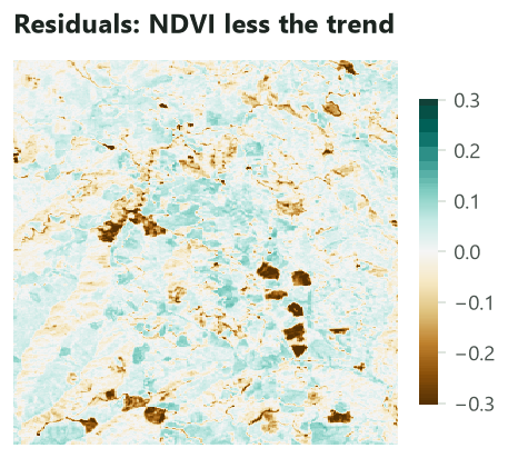
Surface metrics describe variation around a reference. A broad gradient across the map (greener in the north than in the south, say, because of rainfall) is not texture, and left in the map it dominates every metric. The first step is to fit a smooth trend surface (a polynomial in the coordinates of the cells) and keep the residuals, the heights above and below it.
- Click
raster.read(subject Data preparation, or press/and type read) and set path tondvi.tif. Rename itndvi. - With
ndviselected, clicksurface.fit_planein the subject Surface metrics. Leave order atbest. Rename ittrend. - Select
trendand clicksurface.metrics: drag fromtrend'sresidualsport to itsmapinput (not fromplane, the trend itself). Leave metrics empty to compute all 27. - Run to
metricswith Ctrl+Enter: the table of one row shows in the Viewer.
Model file (TOML)
format = "terraflux/1"

[[nodes]]
id = "ndvi"
op = "raster.read"
params = { path = "ndvi.tif" }
note = "Summer NDVI, 30 m."

[[nodes]]
id = "trend"
op = "surface.fit_plane"
inputs = { map = "ndvi.raster" }
params = { order = "best" }
note = "The best polynomial of order 0 to 3; residuals = NDVI less it."

[[nodes]]
id = "metrics"
op = "surface.metrics"
inputs = { map = "trend.residuals" }
note = "A table of one row: a column per metric."
surface.fit_plane gives two maps: plane, the trend fitted, and residuals, the surface without it. Its
order is the degree of the polynomial: 0 a flat plane at the mean (removing only the mean), 1 a tilted
plane, 2 and 3 curved surfaces, up to 6. With best (the default) it fits orders 0 to 3 and keeps the one with the
smallest Bayesian information criterion (BIC, which balances the fit against the number of terms), as
landschaft does (geodiv chooses by the smallest mean absolute residual instead).


surface.metrics' metrics setting takes a name or a list of names: sa, sq, ssk, sku, sv, sph,
smean (amplitude); sdq, sdq6, sdr (hybrid); sds, ssc, s10z (features); sbi, sci, svi, sk,
spk, svk (bearing area curve); sal, str, std, stdi, srw, srwi, shw, sfd (spatial). Leave it
empty for all of them; ask only for the ones you need on large maps, since the spatial ones need Fourier
transforms of the whole map.
Curves and maps behind the numbers#
Three operators give the objects the metrics summarise. Add them after trend, each reading its residuals:
Model file (TOML)
format = "terraflux/1"

[[nodes]]
id = "ndvi"
op = "raster.read"
params = { path = "ndvi.tif" }

[[nodes]]
id = "trend"
op = "surface.fit_plane"
inputs = { map = "ndvi.raster" }
params = { order = "best" }

[[nodes]]
id = "bearing"
op = "surface.bearing"
inputs = { map = "trend.residuals" }
note = "A table: the share of the surface at or above each height."

[[nodes]]
id = "peaks"
op = "surface.peaks"
inputs = { map = "trend.residuals" }
note = "A table of the cells higher than their 8 neighbours."

[[nodes]]
id = "aacf"
op = "surface.aacf"
inputs = { map = "trend.residuals" }
note = "A map of the autocorrelation at every lag, 1 at the centre."
surface.bearinggives the bearing area curve as a table of two columns,bearing(the share of the surface) andheight.surface.peakslists the peaks (or, with valleys = true, the valleys): the cells higher (lower) than their eight neighbours, with their coordinates, value, row and column. On the residuals there are 6,566.surface.aacfgives the autocorrelation function as a map: its centre is the shift of zero (value 1), and each other cell the correlation of the surface with itself shifted by that cell's distance and direction from the centre.
Texture in moving windows#
One row of numbers summarises the whole map. To see where the surface is rough or smooth, compute the metrics in a window around every cell:
- Select
trendand addsurface.window. Connecttrend.residualsto itsmapinput. - Set metrics to
["sa", "sku"]and window to9(9 × 9 cells, 270 m on a side). Leave shape atsquare(orcirclefor a round window). - Run to the node: the result is a stack, one map per metric, named by the metric.
Model file (TOML)
format = "terraflux/1"

[[nodes]]
id = "ndvi"
op = "raster.read"
params = { path = "ndvi.tif" }

[[nodes]]
id = "trend"
op = "surface.fit_plane"
inputs = { map = "ndvi.raster" }
params = { order = "best" }

[[nodes]]
id = "texture"
op = "surface.window"
inputs = { map = "trend.residuals" }
params = { metrics = ["sa", "sku"], window = 9 }
note = "A stack: a map of Sa and a map of Sku."

[[plots]]
id = "plot"
title = "Texture, 9 x 9 cells"
layers = [{ from = "texture.maps" }]
Each cell receives the value the metric would have on the small raster of its window, computed exactly as
surface.metrics computes it on a whole map. Near the edges the window holds fewer cells (those beyond the
map are missing), so the values there rest on less data. To use the texture maps in a species distribution
model, connect the stack to the model's drivers (see Species distributions).
Click a node and press Ctrl+Enter: the Viewer shows a table (click a column to sort it) or a stack's maps. Save output in the Viewer's header writes what it shows to a file, and Plots › Save as a new plot keeps the view with the model.
Make the tables outputs of the model (in the model file, an [outputs.metrics] section with
from = "metrics.table") and add raster.write nodes for the maps; then:
terraflux run texture.toml --out output
The table is written as output/metrics.csv.
Read the results#
The numbers#
The table gives one value per metric. The most useful ones for this map, beside the same metrics of the elevation of the same place (also with its trend removed), so you can see what the numbers mean:
| Metric | Family | Greenness (NDVI residuals) | Elevation residuals (m) | What it says |
|---|---|---|---|---|
| \( S_a \) | amplitude | 0.044 | 79.7 | the mean departure from the trend |
| \( S_q \) | amplitude | 0.064 | 98.8 | the standard deviation of the heights |
| \( S_{sk} \) | amplitude | −1.98 | −0.12 | greenness: a few cells far below the rest |
| \( S_{ku} \) | amplitude | 6.83 | −0.19 | greenness: long tails; elevation: close to normal |
| \( S_{dq} \) | hybrid | 0.044 per cell | 10.5 m per cell | the mean change from a cell to its neighbours |
| \( S_{ds} \) | features | 0.048 per cell | 0.004 per cell | summits per cell: greenness is speckled |
| \( S_{10z} \) | features | 0.67 | 609 | the five highest peaks and five deepest valleys |
| \( S_{al} \) | spatial | 248 m | 577 m | the grain of the texture |
| \( S_{td} \) | spatial | 90° | 135° | the direction the texture is stretched in |
Read the greenness column as a description of the forest: the canopy is mostly even (its \( S_a \) is only 0.044 NDVI) and close to the trend, but a few patches lie far below it: the skewness of −1.98 and the kurtosis of 6.8 say the distribution is a tall peak with a long tail of low values. Those are the brown patches of the residual map. The grain of the texture is about 250 m: two cells further apart than that have nearly unrelated greenness. The elevation, by contrast, has a symmetric, nearly normal distribution of heights around its trend (skewness and kurtosis near 0), few summits, and a coarser grain of almost 600 m: ridges and valleys are larger than the patches of the canopy.

The bearing area curve#
Sort the cells from the highest to the lowest and plot, for every height, the share of the surface at or above it: this is the bearing area curve (the Abbott–Firestone curve of engineers, who used it to know how much of a surface bears a load as it wears). Its top shows the peaks, its middle the core of the surface, its bottom the valleys:
Three numbers summarise the curve. A straight line through its flattest 40 % separates the core (its height range \( S_k \) = 0.10) from the peaks above it (\( S_{pk} \) = 0.09) and the valleys below (\( S_{vk} \) = 0.55). Here the valleys are six times deeper than the peaks are high: a closed canopy interrupted by deep holes, rather than an open one dotted with dense crowns. \( S_{bi} \), \( S_{ci} \) and \( S_{vi} \) are further indices of the curve, from engineering (the bearing index and the core and valley fluid retention).
The texture maps#
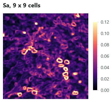
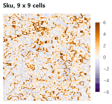
\( S_a \) in a window is high where the window straddles a contrast, so it draws rings around the patches of low greenness, and stays low inside even stands (and inside the patches themselves, if they are larger than the window). \( S_{ku} \) is high where a few extreme cells stand out from an otherwise even window, just outside the rings and around small, scattered gaps. Together they tell apart an even canopy (low \( S_a \)), a canopy with a few gaps (high \( S_{ku} \)) and a broken mosaic (high \( S_a \), low \( S_{ku} \)).
Autocorrelation#


How to report#
Report the variable and its source, the resolution and the extent, how the trend was removed (the order of the polynomial), the metrics with their units, and, for texture maps, the window in cells and in metres. Choose a few metrics from different families rather than all 27: they are strongly correlated within a family (\( S_a \) with \( S_q \), \( S_{dq} \) with \( S_{dr} \)), and a handful from amplitude, distribution and spatial structure say most of what the full set says.
Settings that change the answer#
Removing the trend, or not#
The same metrics on the greenness map without removing its trend:
| Metric | Residuals | Raw NDVI |
|---|---|---|
| \( S_a \) | 0.0437 | 0.0447 |
| \( S_{sk} \) | −1.98 | −1.92 |
| \( S_{al} \) | 248 m | 4,784 m |
| \( S_{ph} \) (highest peak) | 0.149 | 0.836 |
| \( S_{bi} \) | 0.806 | 0.086 |
Amplitude and distribution change little here, because the trend of this map is gentle. The spatial metrics change completely: on the raw map the autocorrelation length is 4.8 km, more than half the map, because the autocorrelation is computed on the heights themselves, and a map whose values all sit around 0.68 looks like itself at any shift. Metrics that measure heights from zero (\( S_{ph} \), \( S_v \), \( S_{mean} \), \( S_{bi} \)) are meaningless unless the surface is centred. Always compute surface metrics on residuals, and say which trend you removed. If the trend is ecologically meaningful (a gradient of rainfall across a region), decide whether it belongs to what you want to measure, and report both.
The grain of the surface#
The autocorrelation length measures the grain of a surface. To see it at work, the script of this tutorial drew
Gaussian random fields with nlm.gaussian_field (200 × 200 cells of 30 m) whose autocorrelation fades over
3 to 48 cells, removed their trend, and measured them:


The first fields behave as expected: a coarser grain, a longer \( S_{al} \). For the coarsest ones it grows more slowly: a polynomial of order 3 on a map only a few grains wide removes part of the structure as "trend". A surface metric can only see structure much smaller than the map. On the raw fields, without removing the trend, \( S_{al} \) was about 3,000 m for all five: half the map, whatever the grain.
The window of a texture map#
The window of surface.window is the scale of the texture you map, exactly as the window of the TPI is the
scale of the landforms in Terrain from an elevation model. Move the slider:
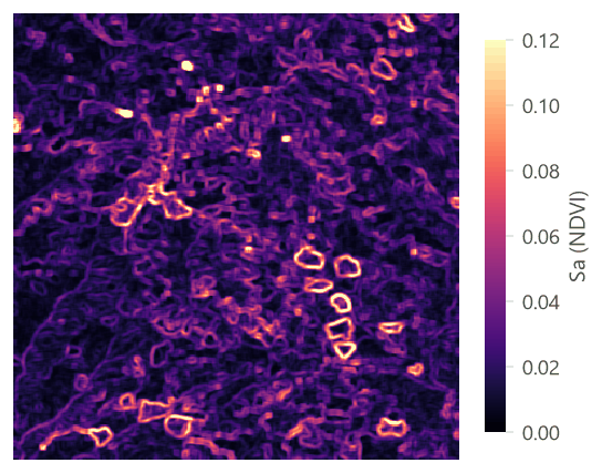
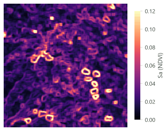


Choose the window from the organism, not from the map: the area over which a bird chooses its territory, the home range of a mammal, the plot size of your field data. Then try one smaller and one larger window, and report how much the results depend on it.
Common pitfalls#
- Metrics of a surface with its trend. The commonest mistake, and the most consequential for the spatial
metrics (above). Remove the trend with
surface.fit_planeand use itsresiduals. - Comparing maps in different units or resolutions. Amplitude metrics are in the units of the variable (NDVI, metres); slopes are per cell. Compare maps of the same variable, sensor and resolution, or use the metrics that are free of units: skewness, kurtosis and \( S_{dr} \), which geodiv computes on heights rescaled to 0–1.
- Noise is roughness. Clouds, stripes, sensor noise and resampling artefacts in imagery add to \( S_a \), \( S_{dq} \) and the summits. Mask and clean the map first, and compare maps processed the same way.
- The texture aspect ratio and the fractal dimension. \( S_{tr} \) divides the shortest decay length of the autocorrelation by the longest one; as geodiv computes it, the longest is the farthest lag of the map whose autocorrelation is below 0.2, which on most maps is near the corner of the map, so \( S_{tr} \) mostly follows \( S_{al} \) and the size of the map (0.036 for the greenness). The fractal dimension \( S_{fd} \) was 2.000 to 2.001 for every surface in this tutorial (it is estimated from how the area of the surface grows as it is measured with finer cells, following Clarke, 1986), from speckled greenness to smooth fields, so it did not tell them apart. Prefer \( S_{al} \) and \( S_{td} \) for spatial structure, and compare \( S_{tr} \) only between maps of the same size.
- Edges of texture maps. Windows near the edge of the map hold fewer cells. Read a margin around the study area and cut it afterwards.
- Too many metrics. Twenty-seven metrics on a few landscapes find patterns by chance. Pick a few, from different families, before looking at the results.
- Patch metrics on maps in longitude and latitude. In the threshold experiment above, the share and the
number of patches are right, but areas (such as
area_mn) would be in square degrees. Reproject before measuring areas of patches (see Terrain from an elevation model).
Going further#
- Terrain from an elevation model: slope, topographic position, ruggedness and heat load, cell by cell.
- Landforms with geomorphons and hilltops protected by Brazil's Forest Code: the terrain's forms.
- Landscape metrics: the patch-mosaic counterpart, for maps of classes.
- Neutral landscape models: Gaussian fields and fractal surfaces of known structure, to test what a metric responds to.
- Species distributions: texture maps as covariates.
- The operators' reference:
surface.metrics,surface.window,surface.fit_plane,surface.bearing,surface.peaks,surface.aacf.
References#
- Kedron, P. J., Frazier, A. E., Ovando-Montejo, G. A., & Wang, J. (2018). Surface metrics for landscape ecology: A comparison of landscape models across ecoregions and scales. Landscape Ecology, 33(9), 1489–1504. https://doi.org/10.1007/s10980-018-0685-1
- McGarigal, K., & Cushman, S. A. (2005). The gradient concept of landscape structure. In J. A. Wiens & M. R. Moss (Eds.), Issues and Perspectives in Landscape Ecology (pp. 112–119). Cambridge University Press.
- McGarigal, K., Tagil, S., & Cushman, S. A. (2009). Surface metrics: An alternative to patch metrics for the quantification of landscape structure. Landscape Ecology, 24(3), 433–450. https://doi.org/10.1007/s10980-009-9327-y
- Smith, A. C., Dahlin, K. M., Record, S., Costanza, J. K., Wilson, A. M., & Zarnetske, P. L. (2021). The geodiv R package: Tools for calculating gradient surface metrics. Methods in Ecology and Evolution, 12(11), 2094–2100. https://doi.org/10.1111/2041-210X.13677
- Clarke, K. C. (1986). Computation of the fractal dimension of topographic surfaces using the triangular prism surface area method. Computers & Geosciences, 12(5), 713–722. https://doi.org/10.1016/0098-3004(86)90047-6
- ISO 25178-2 (2012). Geometrical product specifications (GPS) — Surface texture: Areal — Part 2: Terms, definitions and surface texture parameters. International Organization for Standardization.