Terrain from an elevation model

In this tutorial you take a real digital elevation model of a forested, mountainous corner of south-western Oregon and turn it, node by node, into the terrain variables ecologists use most: slope and aspect, a shaded relief, the topographic position of every cell (ridge, slope or valley), two measures of ruggedness, curvature and the heat load a slope receives from the sun. At the end you will have a model that classifies the landscape into ridges, upper slopes, middle slopes, flats, lower slopes and valleys, you will know how the size of the window changes that classification, and you will know which numbers to report and which mistakes to avoid.

The idea#

An elevation model (a DEM, digital elevation model) is a raster: a grid of square cells, each holding the height of the ground at that place, here in metres above sea level. Elevation itself matters to species (temperature falls by roughly 0.6 °C for every 100 m you climb), but most of what topography does to organisms comes from the shape of the ground around a cell: how steep it is, which way it faces, whether it sits on a crest or in a hollow, whether the ground there is smooth or broken. Those shapes control how much sun a slope receives, where water and cold air drain and collect, how deep the soil is, how exposed a site is to wind, and how hard it is for an animal to cross it. Terrain analysis measures them, cell by cell, from the heights of each cell and its neighbours (Moore et al., 1991).

Enlarge

Every terrain index in this tutorial is a neighbourhood operation: the value of a cell is computed from a small window of cells centred on it. Some indices use a fixed window of 3 × 3 cells (slope, aspect, curvature); others let you choose the window, and with it the scale of the landforms you are measuring.

You can check it by hand on a real cell of the map. The window below is the cell in row 200, column 120 of the elevation model and its eight neighbours:

Enlarge

East minus west: \( (991.1 + 2 \times 983.6 + 967.7) - (956.2 + 2 \times 946.8 + 934.5) = 141.7 \) m, divided by \( 8 \times 30 \) m gives \( \partial z/\partial x = 0.590 \): the ground rises 59 cm for every metre towards the east. South minus north gives \( -89.9 / 240 = -0.375 \): it falls towards the south. The slope is \( \arctan \sqrt{0.590^2 + 0.375^2} = \arctan 0.699 = 35.0° \), and the steepest descent points west and south, an aspect of 237.6°, a south-west-facing slope. Terraflux's slope at that cell is 34.95° and its aspect 237.6°: the same numbers.

Topographic position asks a different question: is the cell higher or lower than the ground around it? Weiss (2001) proposed the topographic position index (TPI), the elevation of a cell minus the mean elevation of a window around it. The same index is used on the sea floor as the bathymetric position index, and Wilson et al. (2007) compared it with other terrain variables at several scales to map habitats on the continental slope; De Reu et al. (2013) studied how it behaves in landscapes that mix flat plains and hills.

The figure below shows what the window size does, along one row of the map. With a window of 5 cells (150 m) the mean follows the ground closely, and the TPI only picks up small bumps; with 41 cells (1.2 km) the mean is a smooth line under the ridges and above the valleys, and the TPI marks the large landforms with differences of up to 100 m.

Enlarge

Two other families of indices complete the toolkit:

• Ruggedness: how broken the ground is. Riley et al. (1999) defined the terrain ruggedness index (TRI) as the square root of the sum of the squared differences in elevation between a cell and its neighbours, in metres; it was designed for habitat studies of mountain wildlife. Sappington et al. (2007) noticed that TRI is mostly a measure of slope (a steep, smooth hillside scores high) and proposed the vector ruggedness measure (VRM), which looks at how much the directions the ground faces vary within a window, so that an even slope, however steep, has a VRM near 0. They developed it for desert bighorn sheep, which seek broken terrain to escape predators.
• Curvature and heat load. Zevenbergen & Thorne (1987) fitted a polynomial surface to the 3 × 3 window and derived from it the profile curvature (along the line of steepest slope: does the slope steepen or flatten downhill?) and the planform curvature (across it: do flow lines converge into a hollow or diverge over a spur?). McCune & Keon (2002) gave equations for the potential direct solar radiation a slope receives in a year from its slope, aspect and latitude, and a heat load index that folds aspect so that south-west slopes, which receive the sun in the warm afternoon, are the hottest in the northern hemisphere.

When to use it#

Terrain indices are among the most common predictors in ecology, because topography is measured everywhere at fine resolution (global elevation models have cells of 30 m) while the climate, soil and moisture it controls are not. Use them to:

• Explain or predict where species occur. Slope, aspect, heat load and topographic position are standard covariates of species distribution models for plants and animals; McCune & Keon (2002) built their heat load index for vegetation scientists, and Sappington et al. (2007) showed that VRM separates the broken terrain used by desert bighorn sheep from terrain that is merely steep.
• Map microclimate and moisture. North-facing slopes and valley bottoms are cooler and wetter; ridges and south-west slopes are hotter and drier. Valley bottoms (negative TPI, concave planform curvature) collect water and cold air.
• Classify landforms. TPI at one or two scales separates ridges, slopes and valleys (Weiss, 2001; De Reu et al., 2013), a common way to stratify field sampling or to map habitats.
• Describe resistance to movement. Slope and ruggedness are frequent ingredients of resistance surfaces for connectivity studies (see Circuit connectivity and Grid distances).

What terrain indices are not: they are not measurements of climate, moisture or soil, only proxies of them, and they inherit every error of the elevation model (artefacts of the sensor, trees and buildings in a surface model, stripes, holes). They also are not texture metrics of other continuous variables such as greenness or canopy height: for those, see the next part, Surface metrics: texture without patches.

What you need#

• An elevation model, as a GeoTIFF or any format GDAL reads. Here: orelevation.tif, the Shuttle Radar Topography Mission (SRTM) elevation of a forested area of south-western Oregon in cells of 1 arc-second (about 30 m), the example data of the R package geodiv and of landschaft (in Terraflux's repository, extern/landschaft/src/landschaft/surface/data/). Save it as elevation.tif next to your model.
• Projected coordinates. The file is in longitude and latitude (EPSG:4326). Terrain indices compare heights in metres with distances, so they need the cells' sides in metres. Terraflux's slope and aspect handle longitude and latitude correctly, but the curvatures and anything built from fixed distances assume a grid in metres, and a cell of 1 arc-second is 30.9 m tall and only 22.6 m wide at 43° north. The first step of the model is therefore a reprojection: a change of the map's coordinate reference system (CRS) to a projected one, here the Universal Transverse Mercator zone 10 north (EPSG:32610), in square cells of 30 m.
• The template, if you want to start from a model that already runs: Templates → Surfaces and uncertainty → Terrain of a surface draws a fractal relief with nlm.mpd and computes most of the indices of this page. Replace its first two nodes by a raster.read of your file to use real data.

Build the model#

Read and reproject the elevation#

format = "terraflux/1"

[[nodes]]
id = "dem"
op = "raster.read"
params = { path = "elevation.tif" }
note = "SRTM elevation, 1 arc-second, longitude and latitude."

[[nodes]]
id = "elevation"
op = "raster.reproject"
inputs = { raster = "dem.raster" }
params = { crs = "EPSG:32610", resolution = 30, extent = [500010, 4760850, 508110, 4771920], resampling = "bilinear" }
note = "Square cells of 30 m in metres; the extent leaves out the edge cells the reprojection cannot fill."

Why each setting: resampling says how the new cells take their values from the old ones. Elevation is a continuous variable, so bilinear (a weighted mean of the four nearest old cells) is right; near (the nearest cell) would create small steps, and steps become false slopes. The extent (west, south, east, north, in metres) is optional: without it the new grid is slightly larger than the data and its last column has no values, because a rectangle in longitude and latitude is not a rectangle in UTM. Cutting it off avoids a line of empty cells along the edge of every index. The result has 369 rows and 270 columns.

Slope, aspect and a shaded relief#

format = "terraflux/1"

[[nodes]]
id = "dem"
op = "raster.read"
params = { path = "elevation.tif" }

[[nodes]]
id = "elevation"
op = "raster.reproject"
inputs = { raster = "dem.raster" }
params = { crs = "EPSG:32610", resolution = 30, extent = [500010, 4760850, 508110, 4771920], resampling = "bilinear" }

[[nodes]]
id = "slope"
op = "surface.terrain"
inputs = { map = "elevation.raster" }
params = { v = "slope" }
note = "Degrees, Horn's 8 neighbours."

[[nodes]]
id = "aspect"
op = "surface.terrain"
inputs = { map = "elevation.raster" }
params = { v = "aspect" }
note = "Degrees clockwise from north."

[[nodes]]
id = "shade"
op = "raster.terrain"
inputs = { raster = "elevation.raster" }
params = { measure = "hillshade" }
note = "The relief lit from the north-west."

surface.terrain computes slope or aspect as the R package terra does (Horn's eight neighbours by default; neighbors = 4 uses only the four that share a side, which is noisier). Its unit is degrees by default; radians are there for formulas that need them. Cells on the edge of the map get no value, because their window is incomplete. raster.terrain runs GDAL's gdaldem on the raster: it gives slope, aspect, hillshade, TRI, TPI and roughness, and is the operator to use on files too large for memory. A hillshade is the relief drawn as if lit by a lamp, by default from the north-west (azimuth 315°) at 45° above the horizon, a grey value from 0 (in shadow) to 255; it is a picture, not a measurement, but nothing shows the shape of the land better, and it makes a good background for other maps. GDAL's options can change the lamp (options = -az 270 -alt 30).

Position, ruggedness and curvature#

format = "terraflux/1"

[[nodes]]
id = "dem"
op = "raster.read"
params = { path = "elevation.tif" }

[[nodes]]
id = "elevation"
op = "raster.reproject"
inputs = { raster = "dem.raster" }
params = { crs = "EPSG:32610", resolution = 30, extent = [500010, 4760850, 508110, 4771920], resampling = "bilinear" }

[[nodes]]
id = "tpi"
op = "surface.tpi"
inputs = { map = "elevation.raster" }
params = { scale = 15 }
note = "Elevation less the mean of 15 x 15 cells."

[[nodes]]
id = "tri"
op = "surface.tri"
inputs = { map = "elevation.raster" }
params = { s = 3 }
note = "Riley's ruggedness, metres."

[[nodes]]
id = "vrm"
op = "surface.vrm"
inputs = { map = "elevation.raster" }
params = { s = 5 }
note = "Dispersion of the ground's normals, 0 to 1."

[[nodes]]
id = "profile"
op = "surface.curvature"
inputs = { map = "elevation.raster" }
params = { type = "profile" }

[[nodes]]
id = "planform"
op = "surface.curvature"
inputs = { map = "elevation.raster" }
params = { type = "planform" }

The settings that matter:

• scale of surface.tpi: with win = rectangle (the default) it is the side of the square window in cells, an odd number; with win = circle it is the radius of a circular window in map units (metres here), at least two cells. Choose it from the size of the landforms that matter to your question: the width of the valleys your species follows, the size of a frost hollow, the distance over which cold air drains. normalize divides the TPI by the standard deviation of the window, which makes values comparable between rugged and gentle areas (De Reu et al., 2013 discuss this variant).
• s of surface.tri and surface.vrm is the window, odd numbers of cells or [rows, columns]. Riley's TRI was defined on 3 × 3 cells; VRM is often computed over several windows to find the scale at which a species responds to ruggedness.
• type of surface.curvature: profile, planform, total (their sum), or McNab's and Bolstad's simpler indices (mcnab, bolstad), both based on how much the cell differs from its neighbours.

surface.hsp, the hierarchical slope position (Murphy et al., 2010), sums standardised TPIs over a range of window sizes (by default 3 to 27 cells in steps of 4), for a single map of position that does not depend on one scale. surface.srr (the surface relief ratio), surface.dissection and surface.spherical_sd are other summaries of the relief within a window.

Heat load#

The last two steps turn the indices into variables ready for an ecological analysis. First, the heat load: add surface.hli and connect aspect's map to its aspect input and slope's map to its slope input. Set scaled to true.

format = "terraflux/1"

[[nodes]]
id = "dem"
op = "raster.read"
params = { path = "elevation.tif" }

[[nodes]]
id = "elevation"
op = "raster.reproject"
inputs = { raster = "dem.raster" }
params = { crs = "EPSG:32610", resolution = 30, extent = [500010, 4760850, 508110, 4771920], resampling = "bilinear" }

[[nodes]]
id = "slope"
op = "surface.terrain"
inputs = { map = "elevation.raster" }
params = { v = "slope" }

[[nodes]]
id = "aspect"
op = "surface.terrain"
inputs = { map = "elevation.raster" }
params = { v = "aspect" }

[[nodes]]
id = "heat"
op = "surface.hli"
inputs = { aspect = "aspect.map", slope = "slope.map" }
params = { scaled = true }
note = "McCune & Keon's equation 1; latitude from the map (43.05 N)."

surface.hli takes the latitude of the centre of the map from its CRS (43.05° N here) unless you give latitude. hemisphere is northern by default, and with force_hemisphere left at true the hemisphere you give is used as it is: for a map south of the equator, set hemisphere = southern (or force_hemisphere = false to let the latitude decide). In the southern hemisphere the warmest slopes face north-west, not south-west. With scaled = true the index is McCune & Keon's potential direct radiation in MJ cm⁻² yr⁻¹; without it, its natural logarithm. equation chooses among McCune & Keon's three equations (the first, the default, uses slope, folded aspect and latitude).

Slope positions#

Then the classification of the landscape into slope positions:

format = "terraflux/1"

[[nodes]]
id = "dem"
op = "raster.read"
params = { path = "elevation.tif" }

[[nodes]]
id = "elevation"
op = "raster.reproject"
inputs = { raster = "dem.raster" }
params = { crs = "EPSG:32610", resolution = 30, extent = [500010, 4760850, 508110, 4771920], resampling = "bilinear" }

[[nodes]]
id = "slope"
op = "surface.terrain"
inputs = { map = "elevation.raster" }
params = { v = "slope" }

[[nodes]]
id = "tpi"
op = "surface.tpi"
inputs = { map = "elevation.raster" }
params = { scale = 15 }

[[nodes]]
id = "position"
op = "raster.calc"
inputs = { t = "tpi.map", s = "slope.map" }
params = { expression = "6 if t > 17.8 else 5 if t > 8.9 else 4 if t >= -8.9 and s > 5 else 3 if t >= -8.9 else 2 if t >= -17.8 else 1" }
note = "1 valley, 2 lower slope, 3 flat, 4 middle slope, 5 upper slope, 6 ridge."

The expression in position is Weiss's (2001) classification, written in raster.calc's language: a cell more than one standard deviation of the TPI above its surroundings is a ridge (6); between half and one standard deviation above, an upper slope (5); within half a standard deviation of its surroundings it is a middle slope (4) if steeper than 5°, a flat (3) if not; between half and one standard deviation below, a lower slope (2); more than one below, a valley (1). The thresholds are numbers in metres because raster.calc works cell by cell: the standard deviation of this map's TPI at 15 cells is 17.8 m (compute it once from the tpi map written to a file, with any statistics tool), so the thresholds are ±17.8 m and ±8.9 m. With another map or another window, recompute them.

format = "terraflux/1"

[[nodes]]
id = "dem"
op = "raster.read"
params = { path = "elevation.tif" }

[[nodes]]
id = "elevation"
op = "raster.reproject"
inputs = { raster = "dem.raster" }
params = { crs = "EPSG:32610", resolution = 30, extent = [500010, 4760850, 508110, 4771920], resampling = "bilinear" }

[[nodes]]
id = "slope"
op = "surface.terrain"
inputs = { map = "elevation.raster" }
params = { v = "slope" }

[[nodes]]
id = "aspect"
op = "surface.terrain"
inputs = { map = "elevation.raster" }
params = { v = "aspect" }

[[nodes]]
id = "shade"
op = "raster.terrain"
inputs = { raster = "elevation.raster" }
params = { measure = "hillshade" }

[[nodes]]
id = "tpi"
op = "surface.tpi"
inputs = { map = "elevation.raster" }
params = { scale = 15 }

[[nodes]]
id = "tri"
op = "surface.tri"
inputs = { map = "elevation.raster" }
params = { s = 3 }

[[nodes]]
id = "vrm"
op = "surface.vrm"
inputs = { map = "elevation.raster" }
params = { s = 5 }

[[nodes]]
id = "profile"
op = "surface.curvature"
inputs = { map = "elevation.raster" }
params = { type = "profile" }

[[nodes]]
id = "planform"
op = "surface.curvature"
inputs = { map = "elevation.raster" }
params = { type = "planform" }

[[nodes]]
id = "heat"
op = "surface.hli"
inputs = { aspect = "aspect.map", slope = "slope.map" }
params = { scaled = true }

[[nodes]]
id = "position"
op = "raster.calc"
inputs = { t = "tpi.map", s = "slope.map" }
params = { expression = "6 if t > 17.8 else 5 if t > 8.9 else 4 if t >= -8.9 and s > 5 else 3 if t >= -8.9 else 2 if t >= -17.8 else 1" }

[[plots]]
id = "plot"
title = "Slope positions"
layers = [{ from = "position.map" }]

terraflux check terrain.toml
terraflux run terrain.toml --out output

Read the results#

Slope. The study area is steep: the mean slope is 18.1° and the steepest cells reach 58.2°. The flat cells are few and lie along the valley floor in the south-east. When you report a slope, give its unit (degrees or percent: 45° is 100 %), the resolution of the elevation model, and the method (Horn's).

Topographic position. The TPI at 450 m ranges from −70 m to +67 m; its standard deviation is 17.8 m. Red cells (positive) draw the crests of the ridges and their spurs; blue cells (negative) draw the stream network, from the main valley in the south-east up into the smallest side valleys. The slope positions derived from it are the map most people find readable: at this scale 15.8 % of the cells are ridges, 15.2 % upper slopes, 38.3 % middle slopes, 1.7 % flats, 14.1 % lower slopes and 15.0 % valleys. These shares are not discoveries about the landscape: thresholds at ±0.5 and ±1 standard deviation put about 15 % of the cells in each tail by construction, whatever the land looks like. What the map shows is where the ridges and valleys are, and that is what you would use to stratify sampling or as a covariate.

Ruggedness. TRI and VRM measure different things, and the data show it. Across the cells of the map, TRI is almost a copy of slope (correlation 0.98), while VRM is nearly independent of it (correlation 0.09): VRM is high only where the ground faces many directions within a short distance, along the crests of the ridges and in the heads of the gullies. The chart samples 500 cells:

If your question is about steepness, use slope; if it is about broken, irregular ground (escape terrain, microhabitats, rock outcrops), VRM separates it from steepness, as Sappington et al. (2007) intended.

Curvature. Both curvatures are in units of 1/m (the inverse of the radius of a curve that fits the ground). In Terraflux, positive values are convex cells and negative values concave ones: on this map both are positively correlated with the TPI (0.56 for profile curvature, 0.51 for planform curvature), as crests stand above their surroundings. Convex profile curvature marks the shoulders where slopes steepen downhill; concave planform curvature marks hollows where flow converges. Programs differ in the sign they give to profile curvature, so check it before comparing values with another study.

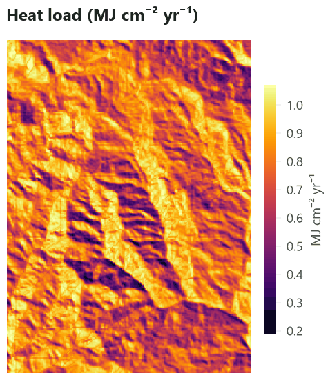
Heat load. Values go from 0.19 to 1.07 MJ cm⁻² yr⁻¹ (mean 0.77). Steep slopes (over 15°) facing south-west average 0.98, those facing north-east 0.47: half the potential radiation, on slopes a few hundred metres apart. That difference is what makes north-east slopes cooler and moister, and in many regions it separates forest types on opposite sides of the same ridge.

How to report. Give the elevation model (source, resolution, date), the projection, the algorithm of each index (Horn for slope and aspect; Zevenbergen & Thorne for curvature; Riley's TRI; Sappington's VRM; McCune & Keon's heat load with the equation number and the latitude), and the window of every index that has one, in cells and in metres. A figure with the hillshade under the index you discuss helps readers see where it is high.

Settings that change the answer#

The window of the TPI is the setting that matters most: it decides what a ridge is. Move the slider to see the slope positions recomputed from the TPI at windows of 3 to 61 cells (90 m to 1.8 km), each with its own thresholds (±0.5 and ±1 standard deviation of that TPI):

Enlarge

Enlarge

PlayTPI window (m)

Three things to notice:

1. The landforms change, not their share. At 90 m, "ridges" are the tops of small bumps scattered over every slope; at 1.8 km they are the main crest lines, several hundred metres wide. The shares stay near 15 % because the thresholds follow the standard deviation.
2. The relief grows with the window. The standard deviation of the TPI rises from 2 m to 64 m: a large window compares a cell with ground far away, which differs more. Never compare TPI values computed with different windows.
3. The edges are lost. A cell whose window reaches beyond the map (or a cell without a value) gets no value, so a window of 61 cells leaves out a border 30 cells (900 m) wide: a third of this small map. Read your elevation model with a margin of at least half the largest window around your study area, and cut it afterwards.

To keep information from several scales, compute the TPI at two windows (one for local landforms, one for large ones, as Weiss did) or use surface.hsp.

The windows of TRI and VRM work the same way: at 3 × 3 cells they describe the roughness of the ground over 90 m; at 15 × 15 cells, over 450 m. A good rule for all of them: try several windows, let the ecological data (the species' locations, the plots' measurements) choose the scale, and report which windows you tried.

Common pitfalls#

• Geographic coordinates. On a map in longitude and latitude, a cell's width in metres shrinks towards the poles. surface.terrain takes it into account (cell widths in metres per row, as terra does): on the original grid it gives a mean slope of 18.5°, close to the 18.1° of the projected map. GDAL's raster.terrain does not: with its usual option -s 111120 (metres per degree) it uses the same scale for both directions, takes the cells to be 37 % wider than they are at this latitude, and gives a mean slope of only 16.1°. Reproject first, as in this tutorial, and both operators agree (18.07° each).
• Resampling with the nearest cell. Reprojecting or resampling elevation with near creates terraces, and the slope between terraces is noise. Use bilinear or cubic for elevation.
• Vertical units. If the elevation is in feet and the cells in metres, every slope is wrong. Check both in the file's description.
• Surface models. Some free "elevation" products measure, in places, the top of the canopy or of buildings rather than the ground (radar models such as SRTM do so partly in dense forest). Clearings then look like pits, and edges of forests like cliffs.
• Edges and holes. Every window that touches the edge of the map or a cell without value is missing. Fill small holes first (raster.fill) and read a margin around the study area.
• Aspect on flat ground. Where the slope is zero, aspect is undefined. Mask flat cells before using aspect, or use heat load, which goes smoothly to the value of flat ground.
• Hemisphere. surface.hli assumes the northern hemisphere unless told otherwise.
• Scale chosen by habit. A 3 × 3 window on a 30 m model and on a 1 m lidar model measure different things. Report windows in metres.

Going further#

• Landforms with geomorphons: name each cell's landform (ridge, slope, valley...) from the terrain seen around it, at the scale of a search radius.
• Hilltops protected by Brazil's Forest Code: the APP de topo de morro of Lei 12.651/2012, hill by hill.
• Surface metrics: texture without patches: describe any continuous surface (greenness, canopy height, the elevation itself) by its roughness, the shape of its distribution and its spatial structure, in one number or in moving windows.
• Species distributions: use slope, heat load and topographic position as covariates.
• Circuit connectivity and Grid distances: slope and ruggedness as resistance to movement.
• The operators' reference: surface.terrain, surface.tpi, surface.tri, surface.vrm, surface.curvature, surface.hli, surface.hsp, surface.trasp, raster.terrain.

References#

• De Reu, J., Bourgeois, J., Bats, M., Zwertvaegher, A., Gelorini, V., De Smedt, P., Chu, W., Antrop, M., De Maeyer, P., Finke, P., Van Meirvenne, M., Verniers, J., & Crombé, P. (2013). Application of the topographic position index to heterogeneous landscapes. Geomorphology, 186, 39–49. https://doi.org/10.1016/j.geomorph.2012.12.015
• Horn, B. K. P. (1981). Hill shading and the reflectance map. Proceedings of the IEEE, 69(1), 14–47. https://doi.org/10.1109/PROC.1981.11918
• McCune, B., & Keon, D. (2002). Equations for potential annual direct incident radiation and heat load. Journal of Vegetation Science, 13(4), 603–606. https://doi.org/10.1111/j.1654-1103.2002.tb02087.x
• Moore, I. D., Grayson, R. B., & Ladson, A. R. (1991). Digital terrain modelling: A review of hydrological, geomorphological, and biological applications. Hydrological Processes, 5(1), 3–30. https://doi.org/10.1002/hyp.3360050103
• Murphy, M. A., Evans, J. S., & Storfer, A. (2010). Quantifying Bufo boreas connectivity in Yellowstone National Park with landscape genetics. Ecology, 91(1), 252–261. https://doi.org/10.1890/08-0879.1
• Riley, S. J., DeGloria, S. D., & Elliot, R. (1999). A terrain ruggedness index that quantifies topographic heterogeneity. Intermountain Journal of Sciences, 5(1–4), 23–27.
• Roberts, D. W., & Cooper, S. V. (1989). Concepts and techniques of vegetation mapping. In Land Classifications Based on Vegetation: Applications for Resource Management (pp. 90–96). USDA Forest Service General Technical Report INT-257.
• Sappington, J. M., Longshore, K. M., & Thompson, D. B. (2007). Quantifying landscape ruggedness for animal habitat analysis: A case study using bighorn sheep in the Mojave Desert. Journal of Wildlife Management, 71(5), 1419–1426. https://doi.org/10.2193/2005-723
• Weiss, A. D. (2001). Topographic position and landforms analysis. Poster presentation, ESRI User Conference, San Diego, CA.
• Wilson, M. F. J., O'Connell, B., Brown, C., Guinan, J. C., & Grehan, A. J. (2007). Multiscale terrain analysis of multibeam bathymetry data for habitat mapping on the continental slope. Marine Geodesy, 30(1–2), 3–35. https://doi.org/10.1080/01490410701295962
• Zevenbergen, L. W., & Thorne, C. R. (1987). Quantitative analysis of land surface topography. Earth Surface Processes and Landforms, 12(1), 47–56. https://doi.org/10.1002/esp.3290120107