Resistance surfaces

Every connectivity model of this site (habitat graphs with least costs, Circuitscape, Omniscape, gdistance's routes) rests on one map: the resistance surface, the cost of moving through every cell for the species. It is also the part of the analysis that rests most on judgement. In this part you build two resistance surfaces for a forest mammal around Hannover, one from land cover classes and one from a habitat suitability, then make the contrasts between classes weaker and stronger, and run Circuitscape between two large forests with each. At the end you will know how resistances are made, which of their properties matter, and how to show readers how much your results depend on them.

The idea#

What a resistance is#

A resistance value says how much a cell costs a moving animal: in energy, time, or risk of death. It is usually relative (forest 1, arable land 20) and expresses three things at once: how willing the animal is to enter the cell, how fast it moves through it, and how likely it is to survive it (Zeller et al., 2012). The map of these values is the landscape as the species sees it; the rest of the model only computes with it.

Zeller et al. (2012) reviewed 96 studies that estimated resistance and grouped the ways of doing it:

Expert opinion: a value per land cover class, from the literature and from people who know the species. The most common, and the least tested; values should be argued and alternatives tried.
Habitat suitability: from a species distribution model, on the idea that animals move most easily where they would live. Easy when a model exists, but a place a species avoids for breeding is not always one it avoids when it moves (Keeley et al., 2017).
Movement data: GPS tracks or detections, with resource or step selection functions fitted to where animals go when they move.
Genetic data: the resistances that make effective resistances or least costs best explain genetic distances between populations (Spear et al., 2010), the use that circuit theory was first built for (McRae & Beier, 2007).

Key idea: what in a resistance matters

Least costs and currents depend on the ratios between resistances, not their scale: multiplying every value by 10 multiplies every cost and effective resistance by 10 and leaves the routes and current maps unchanged. What changes the answer is the contrast between classes (forest 1 against arable 20, or 1 against 400) and the order of the classes. Report both, and test the contrast.

From suitability to resistance#

A habitat suitability \(h\) runs from 0 to 1. The simplest resistance is linear, \(R = 100 - 99\,h\). Keeley et al. (2016) compared such transformations against movement and genetic data and found that a negative exponential often fitted better: resistance stays low until suitability is quite poor, then rises steeply, because animals cross mediocre habitat easily and avoid only the worst.

\[ R = 100 - 99\,\frac{1 - e^{-c\,h}}{1 - e^{-c}} \]

with \(c\) the shape: near 0 it is the linear transformation; at \(c = 8\) or 16, a suitability of 0.3 already has a low resistance.

Keeley et al.'s transformations of a suitability into a resistance from 1 to 100. The larger c, the more of the suitability range is easy to cross.

When to use it#

Always, before any least-cost, circuit or random-walk analysis; and as an analysis in its own right when the question is what limits movement: comparing resistances that explain gene flow or movement data tells which land covers are barriers (Spear et al., 2010).

What you need#

The land cover of the series, clc_100m.tif: CORINE Land Cover around Hannover at 100 m.
A table of resistances per class, with its sources. The example is a generalist forest mammal (the values of least-cost links): forest 1, transitional woodland 2, semi-natural land 5, pasture and mixed farming 10, arable land 20, green urban areas 30, mines and dumps 50, towns, roads and water 100.
Two areas to connect: two of the largest forests, patches 55 (the southern forest, 9,151 ha) and 96 (the forest north-east of the lake, 2,860 ha), 29 km apart.

Build the model#

1. A resistance from classes#

raster.reclassify turns the land cover into the resistance, as in least-cost links. In this landscape it gives 20.6% of the cells a resistance of 1 (forest), 50.4% a resistance of 20 (arable land) and 14.4% a resistance of 100 (towns, roads, water).

The resistance from the land cover classes — The resistance from classes (logarithmic). Forests are pale; arable land purple; towns, roads and water black. The resistance has hard edges: each cell takes the value of its class.

2. A resistance from suitability#

Without a species distribution model, a simple stand-in is the amount of forest around each cell: a cell amid forest is good for a forest mammal, a cell in open farmland far from woods is poor. Two raster.calc nodes make it: l >= 23 and l <= 25 (1 in forest, 0 elsewhere), then nbmean(f, 5), the mean of that map over the 5 × 5 cells (500 × 500 m) around each cell, a suitability from 0 to 1. A third raster.calc applies Keeley's transformation with \(c = 8\):

100 - 99 * (1 - exp(-8 * s)) / (1 - exp(-8))

Resistance from suitability — Suitability

3. Weaker and stronger contrasts#

Two more raster.calc nodes on the class resistance: sqrt(r) (contrasts weakened: forest 1, arable 4.5, towns 10) and r ** 2 (contrasts strengthened: forest 1, arable 400, towns 10,000).

4. The two forests and the current between them#

The focal areas are made from the forest patches, as in the habitat networks series: conn.graph_from_raster and conn.nodes number the patches, conn.to_map paints the numbers on them, and raster.calc keeps patches 55 and 96 as areas 1 and 2: coalesce(1 if i == 55 else 2 if i == 96 else 0, 0) (coalesce gives 0 where the patch map has no value). Then one circuit.pairwise per resistance, with cum_map = true.

Four resistance surfaces from one land cover (classes, weaker and stronger contrasts, suitability), and the current between two forests over the first; the other three run the same way.

Model file (TOML)

format = "terraflux/1"

[[nodes]]
id = "land"
op = "raster.read"
params = { path = "clc_100m.tif" }

[[nodes]]
id = "resistance"
op = "raster.reclassify"
inputs = { map = "land.raster" }
params = { rules = "23 24 25 -> 1\n29 -> 2\n21 26 27 32 35 36 -> 5\n18 20 -> 10\n12 -> 20\n10 11 -> 30\n7 8 9 -> 50\n1 2 3 4 5 6 40 41 -> 100\n* -> 20" }
note = "A resistance per class."

[[nodes]]
id = "weaker"
op = "raster.calc"
inputs = { r = "resistance.map" }
params = { expression = "sqrt(r)" }

[[nodes]]
id = "stronger"
op = "raster.calc"
inputs = { r = "resistance.map" }
params = { expression = "r ** 2" }

[[nodes]]
id = "forest"
op = "raster.calc"
inputs = { l = "land.raster" }
params = { expression = "l >= 23 and l <= 25" }

[[nodes]]
id = "suitability"
op = "raster.calc"
inputs = { f = "forest.map" }
params = { expression = "nbmean(f, 5)" }
note = "The share of forest in the 5 x 5 cells around."

[[nodes]]
id = "from_suitability"
op = "raster.calc"
inputs = { s = "suitability.map" }
params = { expression = "100 - 99 * (1 - exp(-8 * s)) / (1 - exp(-8))" }
note = "Keeley et al.'s transformation, c = 8."

[[nodes]]
id = "graph"
op = "conn.graph_from_raster"
inputs = { map = "land.raster" }
params = { habitat = [23, 24, 25] }

[[nodes]]
id = "patches"
op = "conn.nodes"
inputs = { map = "land.raster" }
params = { habitat = [23, 24, 25] }

[[nodes]]
id = "ids"
op = "conn.to_map"
inputs = { graph = "graph.graph", table = "patches.table" }
params = { column = "id" }

[[nodes]]
id = "two_forests"
op = "raster.calc"
inputs = { i = "ids.map" }
params = { expression = "coalesce(1 if i == 55 else 2 if i == 96 else 0, 0)" }
note = "The southern forest (1) and the north-eastern one (2)."

[[nodes]]
id = "current"
op = "circuit.pairwise"
inputs = { habitat = "resistance.map", points = "two_forests.map" }
params = { cum_map = true }
note = "The current between them over the class resistance."

Read the results#

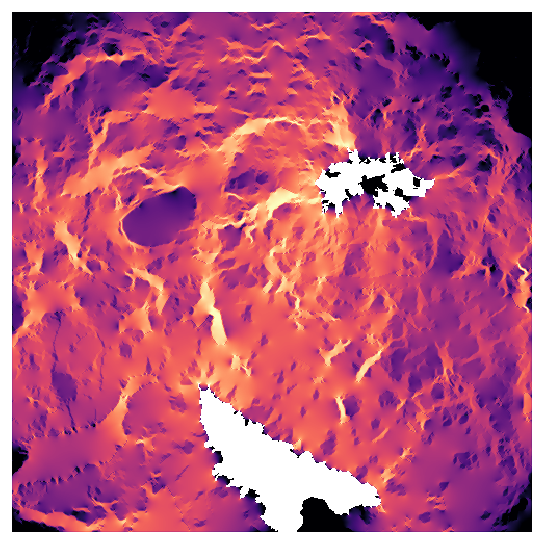
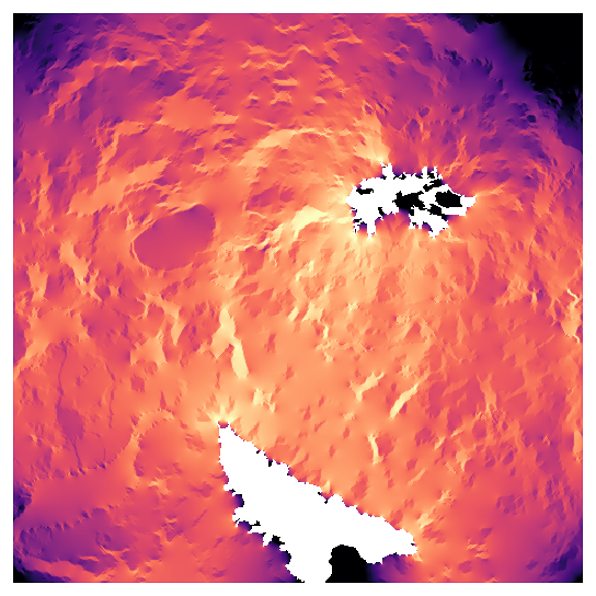
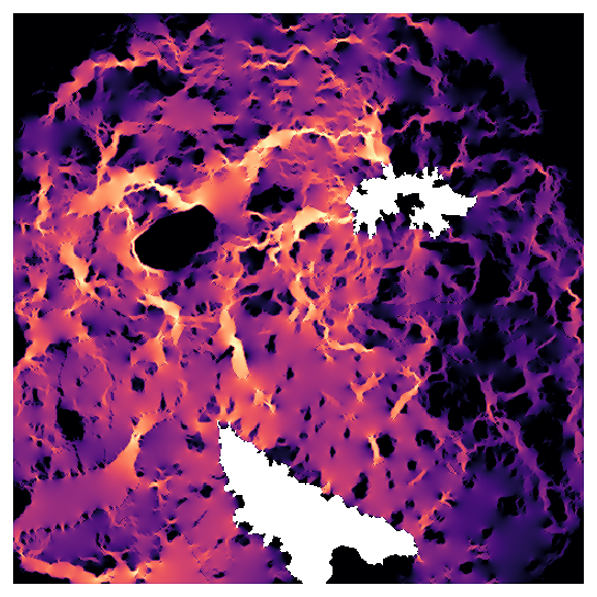
Move the slider between the four resistances. Each map is the current between the two forests (white), on a logarithmic scale from its 1/150 to its largest values; the numbers are the effective resistance between the forests.

Resistance surface Classes — The current between the southern forest and the north-eastern one over four resistance surfaces, each on its own logarithmic scale (bright: most current). The weaker contrasts spread the current over the farmland; the stronger ones squeeze it into narrow channels; the suitability version runs it from wood to wood and ignores the lake.

Resistance surface Weaker (√r) — The current between the southern forest and the north-eastern one over four resistance surfaces, each on its own logarithmic scale (bright: most current). The weaker contrasts spread the current over the farmland; the stronger ones squeeze it into narrow channels; the suitability version runs it from wood to wood and ignores the lake.

What changes and what does not:

The effective resistance changes by two orders of magnitude (1.24 to 105) between the weaker and the stronger versions. Effective resistances are only comparable within one resistance surface: never report them without it, and never compare them between studies that used different values.
The main routes are similar. In all four maps most current runs north from the southern forest through the centre-west of the landscape and turns east to the north-eastern forest, and the east, where Hannover lies, carries little. The order of the classes, shared by the three class-based versions, decides the broad picture.
The concentration changes. With weak contrasts the current spreads almost evenly over farmland; with strong ones it runs in narrow channels along forest and pasture, and pinch points sharpen. A study of pinch points is therefore the most sensitive to the contrast.
The suitability version follows the small woods. Because resistance is low wherever there is some forest nearby, current runs from wood to wood in smooth channels, an effect that the class resistance, which gives a single field between two woods the full cost of arable land, misses. But this stand-in knows only forest: Lake Steinhude and the towns cost no more than a field, and the lake, a clear obstacle in the other three maps, has vanished. A real suitability model would include them.

In the literature

Report the resistance of every class (a table) and where the values came from; for a suitability-based resistance, the model and the transformation. Test at least one alternative (weaker and stronger contrasts, or another source), and say whether the conclusions held. Zeller et al. (2012) and Spear et al. (2010) list what reviewers look for; Keeley et al. (2016) show how to compare transformations against data.

Testing a resistance#

The slider is a sensitivity analysis, and the least a study should do. When data exist, a resistance can be tested rather than only varied:

Against movement data. Overlay GPS fixes or detections on the current maps of several resistances; the better resistance puts more of the observed moves in high-current cells. Zeller et al. (2012) review the statistics (resource and step selection functions) used to fit resistances from movements directly.
Against genetic data. Compute the effective resistance between sampled populations (circuit.pairwise with the populations as focal areas) for each candidate resistance, and correlate it with the genetic distances (with Mantel tests or mixed models that account for the pairs' dependence). The resistance with the strongest relationship is the best supported (Spear et al., 2010; McRae & Beier, 2007).
Against independent knowledge. Do the pinch points match known road-kill sites, wildlife crossings or places where the species is seen crossing? A field check of a few pinch points is cheap and convincing.

Linear features and resolution#

At 100 m, a motorway, a canal or a hedge is either the class of its cell or nothing. Many barriers that matter for movement are linear and narrow: a fenced motorway can stop a deer completely while occupying a fifth of a cell. Two solutions: burn the features into the resistance at the finest resolution available (rasterize the roads with vector.rasterize and take the larger resistance of road and land cover), then resample with the largest value (resampling = "max" keeps the barrier), or keep the analysis at a finer resolution where the feature is wide enough. The same holds for corridors: a hedgerow lost at 100 m cannot channel any current.

Settings that change the answer#

The contrast between classes, above: the strongest effect on pinch points and effective resistances.
The resistance of barriers: 100 for towns lets some current through them; no value (a true barrier) removes the cells from the circuit. Choose by species: towns are not walls for foxes.
The resolution: at 100 m, a hedge, a road or a narrow river disappears into the class around it. Linear features that matter (motorways, fences, rivers) are best burnt into the map at their real resistance before resampling.
The transformation of suitability: linear or exponential, and its \(c\).

Common pitfalls#

Zero or negative values. Circuitscape and the cost operators need positive resistances; the reclassification must give every class a value (* -> ...).
Resistance and conductance confused. circuit.pairwise reads a resistance by default (habitat_is_resistance); circuit.advanced reads a conductance (1 / resistance). Check which an operator expects.
Suitability is not permeability. Animals cross places where they would never settle. If you have movement data, test the suitability-based resistance against it.
Unstated values. A connectivity map without its resistance table cannot be judged or repeated.

Going further#

Part 1: circuit theory, and Part 3: Circuitscape, which uses the class resistance between eight forests.
Species distributions: a real suitability model to start from.
Least-cost links: the same resistance in a habitat graph.
The operators: raster.reclassify, raster.calc, circuit.pairwise.

References#

Keeley, A. T. H., Beier, P., & Gagnon, J. W. (2016). Estimating landscape resistance from habitat suitability: effects of data source and nonlinearities. Landscape Ecology, 31(9), 2151–2162. https://doi.org/10.1007/s10980-016-0387-5
Keeley, A. T. H., Beier, P., Keeley, B. W., & Fagan, M. E. (2017). Habitat suitability is a poor proxy for landscape connectivity during dispersal and mating movements. Landscape and Urban Planning, 161, 90–102. https://doi.org/10.1016/j.landurbplan.2017.01.007
McRae, B. H., & Beier, P. (2007). Circuit theory predicts gene flow in plant and animal populations. Proceedings of the National Academy of Sciences, 104(50), 19885–19890. https://doi.org/10.1073/pnas.0706568104
Spear, S. F., Balkenhol, N., Fortin, M.-J., McRae, B. H., & Scribner, K. (2010). Use of resistance surfaces for landscape genetic studies: considerations for parameterization and analysis. Molecular Ecology, 19(17), 3576–3591. https://doi.org/10.1111/j.1365-294X.2010.04657.x
Zeller, K. A., McGarigal, K., & Whiteley, A. R. (2012). Estimating landscape resistance to movement: a review. Landscape Ecology, 27(6), 777–797. https://doi.org/10.1007/s10980-012-9737-0