

Other land change models, part 3 of 6
FUTURES: urban growth as patches
Simulate the growth of built land with FUTURES, from a development pressure, a potential per subregion and a library of observed patch sizes, calibrate the compactness of its patches and see how the incentive power moves growth between infill and sprawl.
- Level
- Advanced
- Time
- 60 min
Towns and suburbs grow in patches: a housing estate, a shopping centre, a row of houses along a new road. Their growth is driven by what is already built nearby, it varies from one county to the next, and its patches have sizes and shapes that differ from region to region. FUTURES was built to simulate exactly this. In this part you will fit its three pieces on the Plum Island Ecosystems between 1985 and 1991 (a development pressure, a potential in each of two subregions, a library of the sizes of the patches developed), calibrate the compactness of its patches, simulate the eight years from 1991 to 1999, compare them with the map of 1999, and move the setting that decides between infill and sprawl. At the end you will know when FUTURES is the right model for a question about urban growth and how to read what it gives.
The idea#
Where it comes from#
FUTURES (FUTure Urban-Regional Environment Simulation) was developed by Meentemeyer et al. (2013) at North
Carolina State University to project the urbanisation of the fast-growing region around Charlotte, North
Carolina, and its consequences for forests and farmland. Its authors wanted three things models of the time did
not combine: a demand for developed land that comes from the population of each county, a probability of
development that differs between counties, and patches of development whose sizes and shapes are learned from the
patches that really appeared. It has since been rewritten as the open-source GRASS GIS modules r.futures
(Petrasova et al., 2016) and used, for example, to compare conservation strategies under urban growth (Dorning
et al., 2015). Terraflux runs r.futures's algorithms through the landschaft library.
FUTURES models one transition, from undeveloped to developed, in three submodels:
- DEMAND: how many cells each subregion (a county, a municipality) develops each year;
- POTENTIAL: the probability that each undeveloped cell is developed, from a regression per subregion;
- PGA (patch-growing algorithm): where the demand goes, as patches grown from seeds drawn on the potential.
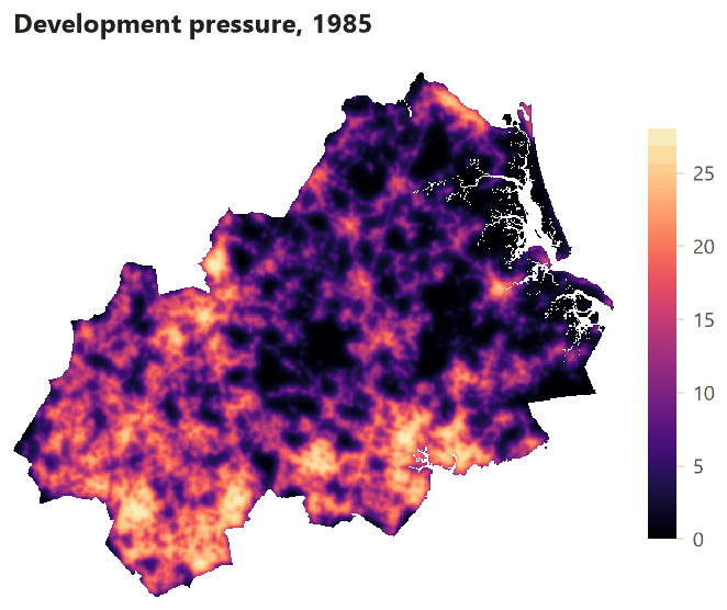
The development pressure#
The best predictor of development is development nearby. FUTURES measures it as a development pressure: for every cell, a sum over the developed cells around it, weighted by their distance.
Key idea: development pressure
With the gravity method,
over the developed cells \(j\) within a circle \(W(i)\) of radius size cells around cell \(i\), \(d_{ij}\)
their distance in cells, \(\gamma\) the decay (1.5 here) and \(s\) a scaling factor (1). A cell surrounded by
development close by has a high pressure; an isolated one, none. As cells are developed during the
simulation, the pressure around them is updated: development attracts development.
The potential#
The probability that an undeveloped cell becomes developed is a logistic function of the pressure and other drivers, with coefficients that may differ between subregions:
Key idea: the potential of a cell
where \(r\) is the subregion of cell \(i\), \(x_k\) its drivers (slope, elevation...) and the \(\beta\)s are
fitted on the cells that were undeveloped at the start of the calibration period: 1 if they were developed by
its end, 0 if not. r.futures.potential fits a mixed-effects regression with an intercept per subregion; here,
for simplicity, a separate logistic regression per subregion (glm.fit).
The patch-growing algorithm#
Every year, each subregion must develop its demand. The PGA draws a seed among the undeveloped cells in
proportion to their potential; a seed is accepted with a probability equal to its potential; from it, a patch
grows to a size drawn from the patch library (the sizes of the patches developed in the calibration period),
adding cells next to the patch with a preference for compact shapes set by the compactness (an exponent of the
distance to the seed, drawn around compactness_mean within compactness_range). The pressure is updated around
every new cell, and the next seed is drawn. The incentive power raises the potential to a power before the
seeds are drawn: above 1 it favours the cells of highest potential, mostly near existing development (infill);
below 1 it flattens the differences and lets development jump into the countryside (sprawl).
When to use it#
FUTURES suits questions about urban and suburban growth: how much farmland or forest a region loses to development, where, and in what patches; how planning policies (infill, zoning, protected land) change it; how population scenarios translate into land. Its strengths are the demand by subregion, the pressure that makes growth self-reinforcing, and patches whose sizes come from data.
It is not a model of several land uses competing (CLUE-S, PLUS), nor of forest transitions (Dinamica EGO): it knows developed and undeveloped only. Choosing a land change model compares the families.
What you need#
- Maps of developed land (1 developed, 0 not, no value outside the study area) at two dates at least: here
the built class (2) of Plum Island's land use maps of 1985, 1991 and 1999, made with
raster.calc(lu == 2). - Drivers of the potential (here
slopeandelevationofpie_drivers.tif). - Subregions: a map of ids (counties). Plum Island has no counties in its data, so the map is cut into a western (1) and an eastern half (2) to show how subregions work.
- A demand per subregion and year: here the yearly trend of 1985-1991 (281 cells in the west, 257 in the east), kept for 1992-1999.

Build the model#
Step 1: the pressure, the potential and the patch library#
Model file (TOML)
format = "terraflux/1"

[[nodes]]
id = "lu1985"
op = "raster.read"
params = { path = "pie_landuse.tif", band = "1985" }

[[nodes]]
id = "lu1991"
op = "raster.read"
params = { path = "pie_landuse.tif", band = "1991" }

[[nodes]]
id = "drivers"
op = "raster.read"
params = { path = "pie_drivers.tif" }

[[nodes]]
id = "counties"
op = "raster.read"
params = { path = "subregions.tif" }

[[nodes]]
id = "dev1985"
op = "raster.calc"
inputs = { lu = "lu1985.raster" }
params = { expression = "lu == 2" }

[[nodes]]
id = "dev1991"
op = "raster.calc"
inputs = { lu = "lu1991.raster" }
params = { expression = "lu == 2" }

[[nodes]]
id = "pressure"
op = "futures.devpressure"
inputs = { developed = "dev1985.map" }
params = { size = 10, method = "gravity", gamma = 1.5, scaling_factor = 1.0 }

[[nodes]]
id = "predictors"
op = "stack.set"
inputs = { stack = "drivers.raster", map = "pressure.map" }
params = { name = "devpressure" }

[[nodes]]
id = "new_west"
op = "raster.calc"
inputs = { a = "dev1985.map", b = "dev1991.map", c = "counties.raster" }
params = { expression = "None if a == 1 or c != 1 else b" }

[[nodes]]
id = "potential_west"
op = "glm.fit"
inputs = { landscape = "new_west.map", drivers = "predictors.stack" }
params = { formulas = { 1 = ["devpressure", "slope", "elevation"] } }

[[nodes]]
id = "library"
op = "futures.patch_library"
inputs = { start = "dev1985.map", end = "dev1991.map", subregions = "counties.raster" }
params = { per_subregion = true }
- The maps (nodes 1 to 4): the land use of 1985 and 1991, the drivers and the subregions.
- Developed or not (nodes 5 and 6):
raster.calcwithlu == 2gives 1 for built land, 0 for the rest, and no value outside the study area. - The pressure (node 7,
futures.devpressure):sizeis the radius of the window in cells (10, about 1 km),methodthe decay (gravity,occurrenceorkernel),gammaandscaling_factoras in the formula. - The predictors (node 8,
stack.set): the pressure added to the drivers' stack under the namedevpressure, so that the regression can use it. - What to explain (node 9): only the cells of the west that were undeveloped in 1985, with their state in 1991 (1 developed since, 0 still undeveloped); the others get no value and are left out of the fit.
- The potential (node 10,
glm.fit): a logistic regression of that map ondevpressure,slopeandelevation. The east has its own (new_east,potential_east). - The library (node 11,
futures.patch_library): the patches developed between the two maps (groups of new cells joined by their four neighbours), their sizes in cells, one list per subregion withper_subregion = true.
The fitted coefficients:
| Subregion | Intercept | Pressure | Slope | Elevation |
|---|---|---|---|---|
| West | −3.235 | 0.066 | −0.035 | 0.0003 |
| East | −4.223 | 0.132 | −0.029 | 0.0043 |
In both halves the pressure raises the potential and the slope lowers it, but the east responds twice as strongly to the pressure: its development clings more closely to existing development. This is why subregions matter.
Step 2: calibrate the compactness#
The library gives the sizes; the shape is set by the compactness. futures.calibrate (r.futures.calib)
simulates the calibration period with every combination of compactness_means, compactness_ranges and
discount_factors, repeat times each, and compares the simulated patches with the observed ones: the histograms
of their areas and of their compactness (perimeter / (2√(π area))), by a chi-square distance. It ranks the
combinations by the mean of the two errors. Tried here: means 0.1, 0.3, 0.5, 0.7 and 0.9, ranges 0.05 and 0.3,
four repeats each:
| Compactness mean | Range | Area error | Compactness error | Combined |
|---|---|---|---|---|
| 0.7 | 0.3 | 0.809 | 0.498 | 0.654 |
| 0.3 | 0.3 | 0.662 | 0.721 | 0.692 |
| 0.9 | 0.05 | 0.695 | 0.836 | 0.765 |
| 0.9 | 0.3 | 0.677 | 0.855 | 0.766 |
| 0.5 | 0.05 | 0.812 | 0.744 | 0.778 |
(the errors are relative to the largest of each; the full table is calibration.csv). The best, a mean of 0.7 and a range of 0.3, is used below. The ranking is not sharp: with four repeats, the first two are close. More repeats narrow it.
Step 3: simulate 1991 to 1999#
Model file (TOML)
format = "terraflux/1"

[[nodes]]
id = "land"
op = "raster.read"
params = { path = "pie_landuse.tif", band = "1991" }

[[nodes]]
id = "end"
op = "raster.read"
params = { path = "pie_landuse.tif", band = "1999" }

[[nodes]]
id = "drivers"
op = "raster.read"
params = { path = "pie_drivers.tif" }

[[nodes]]
id = "counties"
op = "raster.read"
params = { path = "subregions.tif" }

[[nodes]]
id = "developed"
op = "raster.calc"
inputs = { lu = "land.raster" }
params = { expression = "lu == 2" }

[[nodes]]
id = "pressure"
op = "futures.devpressure"
inputs = { developed = "developed.map" }
params = { size = 10, method = "gravity", gamma = 1.5, scaling_factor = 1.0 }

[[nodes]]
id = "futures"
op = "futures.simulation"
inputs = { landscape = "developed.map", pressure = "pressure.map", drivers = "drivers.raster", subregions = "counties.raster", seed = 1 }
params = { potential = { ids = [1, 2], intercept = [-3.234651, -4.223066], devpressure = [0.06569, 0.132427], predictors = ["slope", "elevation"], coefficients = [[-0.035282, 0.000257], [-0.028677, 0.004273]] }, demand = { subregions = [1, 2], rows = [[281, 257], [281, 257], [281, 257], [281, 257], [281, 257], [281, 257], [281, 257], [281, 257]], years = [1992, 1993, 1994, 1995, 1996, 1997, 1998, 1999] }, patch_sizes = { ids = [1, 2], lists = [[1, 1, 1, 2, 3, 5, 9], [1, 1, 2, 2, 4, 7, 12]] }, neighborhood = 10, approach = "gravity", gamma = 1.5, scaling_factor = 1.0, discount_factor = 1.0, compactness_mean = 0.7, compactness_range = 0.3, num_neighbors = 4, seed_search = "probability", incentive_power = 1.0 }
futures.simulation (r.futures.simulation) is one node that runs every year itself; it is not built from a
loop, because its pieces (the pressure updated around every new cell, the seeds, the patches) are intertwined
within a year. Its inputs: landscape (developed or not at the start), pressure (at the start, with the same
settings as the potential was fitted with), drivers (the predictors by name), subregions and seed. Its
settings:
potential: the coefficients,{ ids, intercept, devpressure, predictors, coefficients }, a value per subregion (copied from the two regressions above);demand:{ subregions, rows, years }, a row per year with the cells of each subregion;patch_sizes: the library (futures.patch_library's output,{ ids, lists });- the pressure's
neighborhood,approach,gammaandscaling_factor(the same as node 6); - the PGA's
compactness_mean,compactness_range,discount_factor(multiplies the patch sizes),num_neighbors(4 or 8) andseed_search; incentive_power(1: neither infill nor sprawl favoured).
It also takes zoning, restrictions and FUTURES' flood submodel (climate, with catchments, flood maps, damage
and adaptation), not used here. Its outputs: maps (developed or not after each year), development (the year
each cell was developed) and info (per year and subregion, the cells developed and the demand carried over when
it could not be met: overflow).
Read the results#
Eight years#


Each subregion meets its demand every year (with a few cells carried to the next year when a patch overshoots,
the overflow columns of info).
Against 1999#


validate.futures (r.futures.validation) compares the simulated map of 1999 with the observed one (both 0/1),
from the map of 1991: a figure of merit of 0.034, kappa simulation of 0.020, a quantity disagreement of
0.006 and an allocation disagreement of 0.053. The figure of merit is as low as Dinamica EGO's on the same landscape
(Validating a simulation):
Plum Island's new development is scattered in small patches that no model with these drivers places cell by cell.
The quantity disagreement has a clear cause: the trend of 1985-1991 asked for 4,304 new cells, while 3,105 were
developed between 1991 and 1999. Growth slowed in the 1990s; a demand from population projections, as FUTURES
intends, would have done better than a trend.
What to report#
The demand of each subregion and its source; the pressure's settings; the potential's coefficients per subregion; the patch library (its period, the number and sizes of patches); the calibrated compactness and how it was chosen; the incentive power; the validation against an observed map; replicates (several seeds).
Settings that change the answer#
The incentive power: infill or sprawl#


From 0.25 to 1 the share of new development that touches the development of 1991 rises from 53% to 77%: the
incentive power is FUTURES' lever for policies of compact growth. At 2, and more so at 4, something else happens:
the potentials, raised to the power, become so small that few seeds are accepted, and the simulation fails to
meet the demand (1,166 of 4,304 cells at 2; 16 at 4), carrying the rest over year after year (negative
overflow in info). Read info after every run with an incentive power above 1, and if the demand is not met,
raise the potential (a larger scaling factor of the pressure) or keep the power lower.
Other settings#
- The pressure's radius, decay and scaling: they must be the same in
futures.devpressure(the potential's fit) and in the simulation, or the coefficients no longer apply. - The patch library: a library from a period of large developments makes large patches;
discount_factorscales the sizes (below 1, smaller patches). - The demand: the most consequential choice, and the one validation exposed here.
Common pitfalls#
- Fitting the potential on all cells. It must be fitted on the cells undeveloped at the start, with their state at the end; developed cells would teach the model where development is, not where it appears.
- A pressure computed differently in the fit and in the simulation.
- Subregions with no development in the calibration period: their regression cannot be fitted; merge them.
- Ignoring
overflow: a demand not met is a silent failure of the scenario. - One run. The PGA is stochastic: run replicates (Calibration and many runs).
Going further#
- MOLUSCE, the next part, and PLUS, the other patch-generating models.
- A demand per region: subregions in the other models.
- Validating a simulation.
- The operators:
futures.devpressure,futures.patch_library,futures.calibrate,futures.simulation,validate.futures.
References#
- Dorning, M. A., Koch, J., Shoemaker, D. A., & Meentemeyer, R. K. (2015). Simulating urbanization scenarios reveals tradeoffs between conservation planning strategies. Landscape and Urban Planning, 136, 28–39. https://doi.org/10.1016/j.landurbplan.2014.11.011
- Meentemeyer, R. K., Tang, W., Dorning, M. A., Vogler, J. B., Cunniffe, N. J., & Shoemaker, D. A. (2013). FUTURES: multilevel simulations of emerging urban–rural landscape structure using a stochastic patch-growing algorithm. Annals of the Association of American Geographers, 103(4), 785–807. https://doi.org/10.1080/00045608.2012.707591
- Petrasova, A., Petras, V., Van Berkel, D., Harmon, B. A., Mitasova, H., & Meentemeyer, R. K. (2016). Open source approach to urban growth simulation. The International Archives of the Photogrammetry, Remote Sensing and Spatial Information Sciences, XLI-B7, 953–959. https://doi.org/10.5194/isprs-archives-XLI-B7-953-2016