

Ecosystem services with InVEST, part 4 of 8
Annual water yield
InVEST's annual water yield model in Terraflux - the water balance of every cell on Budyko's curve, the seasonality constant Z, the yield of each watershed, what people consume, the realized supply and its value as hydropower, and what a land use scenario does to them.
- Level
- Intermediate
- Time
- 50 min
- 11. The ideas
- 22. Carbon
- 33. Habitat quality
- 44. Water yield
- 55. Sediment
- 66. Nutrients
- 77. Seasonal water
- 88. Pollination
Of the rain that falls on a watershed in a year, part returns to the air through the leaves and the soil, and the rest leaves as streamflow and groundwater: the water yield, the water a town, a farm or a reservoir downstream can use. Land use changes the split, because forests and crops evaporate different amounts. In this tutorial you will build InVEST's annual water yield model in Terraflux on Ribeirão Claro: the maps of potential and actual evapotranspiration and of yield, the yield of each watershed, the water people consume, the supply that remains and what it is worth to a hydropower plant. At the end you will know how the model splits the rain, which parameter matters most, and what the model cannot say about water.
The idea#
Over a year, and over a whole catchment, the water balance is simple: what falls as precipitation \(P\) either evaporates (from soil, water and leaves, and through the plants: together the actual evapotranspiration, AET) or leaves as yield, \(Y = P - \text{AET}\) (storage in the soil and aquifers changes little from one average year to the next). The hard part is AET. It cannot exceed the water available (\(P\)) nor the energy available to evaporate it, measured as the potential evapotranspiration PET, the evaporation of a well-watered surface. Budyko (1974) noticed that catchments of the world fall on a curve between those two limits: wet climates (PET much smaller than \(P\)) evaporate almost their PET and are energy limited, dry ones (PET larger than \(P\)) evaporate almost all their rain and are water limited.
Fu (1981) and Zhang et al. (2004) wrote the curve with one parameter, \(\omega\), that sets how close a catchment gets to the limits: the larger \(\omega\), the more of its rain the vegetation manages to evaporate. Donohue et al. (2012) linked \(\omega\) to things you can map: the water the soil holds for roots, and how the rain is spread over the year. InVEST's model applies the curve cell by cell.
Key idea: Budyko's curve in Fu and Zhang's form
For a cell \(x\) of a class with vegetation,
with the potential evapotranspiration \(\text{PET}_x = K_c\,\text{ET}_{0,x}\) (the reference evapotranspiration \(\text{ET}_0\) of the climate times the class's crop coefficient \(K_c\)), and
where AWC is the water available to the plants (mm), PAWC the plant available water content of the soil (the share of its volume between field capacity and wilting point), the soil depth is the depth to the layer that stops roots, and \(Z\) the seasonality constant, which grows with the number of rain events in a year. Classes without vegetation (water, towns) evaporate \(\min(K_c\,\text{ET}_0, P)\). The yield is \(Y_x = P_x - \text{AET}_x\).

A worked cell: rain 1,500 mm, \(\text{ET}_0\) 1,100 mm, soil 1,500 mm deep with a PAWC of 0.15, \(Z = 10\). As forest (\(K_c = 1.0\), roots 5,000 mm), \(\text{AWC} = \min(5000, 1500) \times 0.15 = 225\) mm, \(\omega = 10 \times 225/1500 + 1.25 = 2.75\), \(\text{PET}/P = 0.733\), and the curve gives \(\text{AET}/P = 0.596\): 893 mm evaporate and 607 mm are yielded. As pasture (\(K_c = 0.75\), roots 1,500 mm) the soil still limits the roots (\(\omega = 2.75\)), but \(\text{PET}/P = 0.55\) and \(\text{AET}/P = 0.484\): 775 mm are yielded, 168 mm more.
From supply to service and value#
The yield is a supply. With a demand table (the water each class consumes, in m³ per year and cell) the model subtracts consumption in each watershed to give the realized supply, the water that reaches the outlet. With a valuation table it turns the realized supply into the energy a hydropower plant at the outlet would produce and its net present value:
where \(V\) is the realized supply (m³ / year), \(\beta\) the turbine efficiency, \(\gamma\) the fraction of the inflow used to generate power, \(h\) the head of the dam (m), 0.00272 the kWh produced by a cubic metre falling one metre, \(p_e\) the price of a kWh, \(TC\) the annual cost of running the plant, \(T\) its remaining life in years and \(r\) the discount rate.
When to use it#
- Scenarios: how much more (or less) water a watershed yields if its forest becomes pasture, or its pasture plantation. Eucalyptus, with deep roots and a high \(K_c\), is a classic case.
- Who provides and who uses water: the yield of each sub-watershed against the consumption in it, for water funds and payments for watershed services.
- Hydropower: the energy and value of the water that reaches a reservoir.
What it is not: the model works with annual averages. It says nothing about floods or dry seasons, about
when the water arrives, about groundwater (it does not separate surface and groundwater, nor model their
exchanges), or about water quality. A forest that yields less water in a year may still keep more flow in the dry
season by letting the rain soak in; the model cannot tell. For daily flows use a process model such as SWAT+
(swat.run). Check its numbers against measured flows where you can: Redhead et al. (2016) found, in 22
British catchments, that the fit depended mostly on the input data (within about 10% of the measured flow for most
catchments with national data, much worse with global data). Hamel and Guswa (2015), in a basin of North
Carolina, found that the errors that mattered most were those of the climate inputs, above all the annual
precipitation, and of \(Z\).
What you need#
All rasters on the grid of the land use map, projected in metres:
| Input | File | Unit | Where it comes from |
|---|---|---|---|
lulc |
lulc_2020.tif |
class codes | your land use map |
precipitation |
precipitation.tif |
mm / year | interpolated rain gauges, WorldClim, CHIRPS |
eto |
eto.tif |
mm / year | reference evapotranspiration (FAO's Penman-Monteith), from climate data |
depth |
depth.tif |
mm | depth to the layer that stops roots, from a soil map |
pawc |
pawc.tif |
0 to 1 | plant available water content, from soil texture |
watersheds |
watersheds.gpkg |
polygons with ws_id |
delineated from the DEM (hydro.watersheds) |


The biophysical table, by class: lucode, lulc_veg (1 for vegetation, which follows Budyko's curve; 0
for water, towns, wetlands), root_depth (mm, used only when lulc_veg is 1) and kc. The values here are
illustrative:
| lucode | class | lulc_veg | root_depth | kc |
|---|---|---|---|---|
| 1 | Forest | 1 | 5000 | 1.0 |
| 2 | Pasture | 1 | 1500 | 0.75 |
| 3 | Cropland | 1 | 1200 | 0.7 |
| 4 | Eucalyptus | 1 | 6000 | 1.0 |
| 5 | Urban | 0 | 1 | 0.3 |
| 6 | Water | 0 | 1 | 1.0 |
Optional: sub-watersheds (polygons with subws_id); a demand table (lucode, demand in m³ per year and
cell: here 900 for the town, 150 for irrigated cropland, 5 for pasture's cattle, 0 for the rest); a valuation
table by watershed (ws_id, efficiency, fraction, height, kw_price, cost, time_span, discount).
Build the model#
Step 1: the water balance#
- Add five
raster.readnodes:lulc_2020.tif,precipitation.tif,eto.tif,depth.tif,pawc.tif. Rename each after its content. - Add a
table.readnode forbiophysical_wy.csv. - Add
services.water_yield(subject Ecosystem services) and connect each map to its input of the same name, and the table tobiophysical. - Set
seasonality(\(Z\)) to 10 in the Node pane, and run.
Model file (TOML)
format = "terraflux/1"

[[nodes]]
id = "lulc"
op = "raster.read"
params = { path = "lulc_2020.tif" }

[[nodes]]
id = "biophysical"
op = "table.read"
params = { path = "biophysical_wy.csv" }
note = "lucode, lulc_veg, root_depth, kc."

[[nodes]]
id = "precipitation"
op = "raster.read"
params = { path = "precipitation.tif" }

[[nodes]]
id = "eto"
op = "raster.read"
params = { path = "eto.tif" }

[[nodes]]
id = "depth"
op = "raster.read"
params = { path = "depth.tif" }

[[nodes]]
id = "pawc"
op = "raster.read"
params = { path = "pawc.tif" }

[[nodes]]
id = "water"
op = "services.water_yield"
inputs = { lulc = "lulc.raster", biophysical = "biophysical.table", precipitation = "precipitation.raster", eto = "eto.raster", depth = "depth.raster", pawc = "pawc.raster" }
params = { seasonality = 10 }
The node gives four maps, in mm per year: pet (\(K_c\,\text{ET}_0\)), aet, wyield and fractp (AET / P,
0 to 1). Cells with no rain are left out, as InVEST leaves them.
Step 2: watersheds, demand and value#
- Add
vector.readnodes forwatersheds.gpkgandsubwatersheds.gpkgand connect them towatershedsandsubwatersheds. - Add
table.readnodes fordemand.csvandvaluation.csvand connect them todemandandvaluation. The valuation needs the demand (it values the realized supply), and both need the watersheds.
Model file (TOML)
format = "terraflux/1"

[[nodes]]
id = "lulc"
op = "raster.read"
params = { path = "lulc_2020.tif" }

[[nodes]]
id = "biophysical"
op = "table.read"
params = { path = "biophysical_wy.csv" }

[[nodes]]
id = "watersheds"
op = "vector.read"
params = { path = "watersheds.gpkg" }

[[nodes]]
id = "subwatersheds"
op = "vector.read"
params = { path = "subwatersheds.gpkg" }

[[nodes]]
id = "demand"
op = "table.read"
params = { path = "demand.csv" }

[[nodes]]
id = "valuation"
op = "table.read"
params = { path = "valuation.csv" }

[[nodes]]
id = "water"
op = "services.water_yield"
inputs = { lulc = "lulc.raster", biophysical = "biophysical.table", watersheds = "watersheds.vector", subwatersheds = "subwatersheds.vector", demand = "demand.table", valuation = "valuation.table" }
params = { seasonality = 10 }
note = "precipitation, eto, depth and pawc as in step 1"

[[nodes]]
id = "write"
op = "table.write"
inputs = { table = "water.watershed_table" }
params = { path = "watersheds_2020.csv" }
Now the node also gives demand_map (each cell's consumption, m³ per year), watershed_table and
subwatershed_table.

Read the results#
The maps#


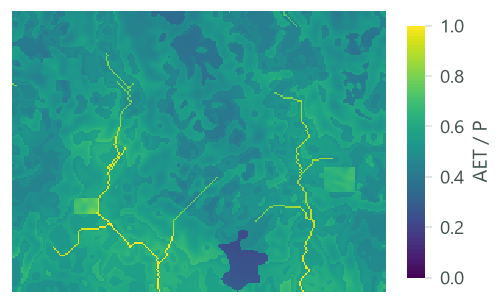

| Class | Rain (mm) | AET (mm) | Yield (mm) | AET / P |
|---|---|---|---|---|
| Forest | 1,563 | 852 | 711 | 0.55 |
| Pasture | 1,467 | 765 | 702 | 0.53 |
| Cropland | 1,509 | 704 | 806 | 0.47 |
| Eucalyptus | 1,503 | 956 | 547 | 0.64 |
| Urban | 1,418 | 365 | 1,053 | 0.26 |
| Water | 1,376 | 1,230 | 146 | 0.9 |
This table shows a trap of reading the maps: a class's yield mixes the effect of the class with the effect of where it grows. To isolate the class, compare scenarios on the same climate (below), not classes in one map.
The watersheds#
| Watershed | Rain (mm) | AET (mm) | Yield (mm) | Yield (Mm³) | Consumed (Mm³) | Realized supply (Mm³) | Energy (MWh) | NPV (thousands) |
|---|---|---|---|---|---|---|---|---|
| 1 | 1,481.6 | 792.7 | 688.9 | 12.59 | 0.56 | 12.02 | 627.9 | 401.4 |
| 2 | 1,506 | 797.7 | 708.3 | 8.77 | 0.56 | 8.21 | 429 | 190.2 |
The columns: the means of rain (precip_mn), PET, AET and yield (wyield_mn) over the cells of the watershed,
in mm; the volume of yield (wyield_vol, m³: the mean yield times the area of the polygon); with a demand, the
consumption (consum_vol, m³; consum_mn, m³ per cell) and the realized supply (rsupply_vl, m³;
rsupply_mn, m³ per cell); with a valuation, the energy (hp_energy, kWh per year) and its net present value
(hp_val). The table of the sub-watersheds has the same columns without the valuation:
| Sub-watershed | Rain (mm) | Yield (mm) | Yield (Mm³) | Consumed (Mm³) | Realized supply (Mm³) |
|---|---|---|---|---|---|
| 1 | 1,564.3 | 760.9 | 6.12 | 0.18 | 5.94 |
| 2 | 1,416.5 | 632.2 | 6.46 | 0.38 | 6.08 |
| 3 | 1,572.2 | 758.8 | 4.14 | 0.15 | 3.99 |
| 4 | 1,453.8 | 668.4 | 4.63 | 0.4 | 4.22 |
Reporting water yield
Report the sources of \(P\), \(\text{ET}_0\) and the soils, the biophysical table, \(Z\) and how you chose it, and the yield (mm and m³) of each watershed for each scenario. Compare with measured flows where gauges exist, and say how far apart they are.
The scenario of 2040#
Run the same model with lulc_2040.tif:

| Watershed | Quantity | 2020 | 2040 |
|---|---|---|---|
| 1 | Water yield (million m³) | 12.585 | 13.061 |
| 1 | Consumption (million m³) | 0.561 | 1.037 |
| 1 | Realized supply (million m³) | 12.024 | 12.024 |
| 1 | Hydropower (MWh / year) | 627.935 | 627.967 |
| 1 | Hydropower, net present value (millions) | 0.401 | 0.401 |
| 2 | Water yield (million m³) | 8.77 | 9.168 |
| 2 | Consumption (million m³) | 0.555 | 1.145 |
| 2 | Realized supply (million m³) | 8.215 | 8.024 |
| 2 | Hydropower (MWh / year) | 429.025 | 419.02 |
| 2 | Hydropower, net present value (millions) | 0.19 | 0.18 |
This is the value of going from supply to service: the yield alone says the scenario is good for water, the realized supply says the gain goes to the new consumers, not to the reservoir.
Settings that change the answer#
The seasonality constant Z#
\(Z\) is the model's only free parameter, and the one to calibrate. InVEST's guide (Natural Capital Alliance, 2026) gives its typical range as 1 to 30 and, after Donohue et al. (2012), suggests estimating it as \(0.2\,N\), where \(N\) is the number of rain events in a year: a place with 50 rain events would have \(Z \approx 10\). Where gauges exist, choose the \(Z\) whose yield best matches the measured flow.


The yield of the landscape halves from \(Z = 1\) to \(Z = 30\), and the difference between classes changes too: at \(Z = 1\) forest yields more than pasture, at \(Z = 30\) much less. So \(Z\) can change not only how much water a scenario yields but whether it yields more or less than another. Report \(Z\), and test a range.
Precision#
InVEST computes with the type of its rasters: 32-bit floating point numbers for float32 files, 64-bit for
float64 ones. Terraflux does the same by default (precision = "auto": 64-bit when a raster holds a value that 32
bits cannot), so that its maps are InVEST's bit for bit; float32 or float64 force one. The difference is far
below anything that matters: here 0.0003 mm at most.
Common pitfalls#
- Annual values. \(P\) and \(\text{ET}_0\) are annual totals (mm per year), not monthly means.
- Depth in millimetres. Soil depth and root depth are in mm; a soil map in cm or m gives a soil 10 or 1,000 times too thin.
- PAWC as a percentage. It is a fraction from 0 to 1.
lulc_vegfor towns and water. Mark them 0, or the model sends them along Budyko's curve with their roots.- Watersheds without
ws_id. The polygons need the attribute (subws_idfor the sub-watersheds); the operator says which is missing. - Demand per cell. The demand is in m³ per year per cell, so it depends on the size of the cells: a demand per hectare must be multiplied by the area of a cell (0.09 ha for 30 m).
- Reading more yield as better. More annual yield can mean more erosion and floods, and the model cannot see the dry season.
Going further#
- Sediment delivery ratio, the next part: the same watersheds and the soil they lose.
- Ecosystem service models: the ideas for the series' models together.
- Seasonal water yield, part 7: when the water arrives, monthly quickflow from the curve number, recharge and dry-season baseflow.
- Monte Carlo uncertainty to carry the uncertainty of \(Z\) and the tables into the yield.
- The operator's reference:
services.water_yield,hydro.watersheds.
References#
- Budyko, M. I. (1974). Climate and Life. Academic Press.
- Donohue, R. J., Roderick, M. L., & McVicar, T. R. (2012). Roots, storms and soil pores: Incorporating key ecohydrological processes into Budyko's hydrological model. Journal of Hydrology, 436–437, 35–50. https://doi.org/10.1016/j.jhydrol.2012.02.033
- Fu, B. P. (1981). On the calculation of the evaporation from land surface (in Chinese). Scientia Atmospherica Sinica, 5, 23–31.
- Hamel, P., & Guswa, A. J. (2015). Uncertainty analysis of a spatially explicit annual water-balance model: case study of the Cape Fear basin, North Carolina. Hydrology and Earth System Sciences, 19(2), 839–853. https://doi.org/10.5194/hess-19-839-2015
- Natural Capital Alliance. (2026). InVEST 3.20.2 User's Guide: Annual water yield. https://storage.googleapis.com/releases.naturalcapitalproject.org/invest-userguide/latest/en/annual_water_yield.html
- Redhead, J. W., Stratford, C., Sharps, K., Jones, L., Ziv, G., Clarke, D., Oliver, T. H., & Bullock, J. M. (2016). Empirical validation of the InVEST water yield ecosystem service model at a national scale. Science of the Total Environment, 569–570, 1418–1426. https://doi.org/10.1016/j.scitotenv.2016.06.227
- Zhang, L., Hickel, K., Dawes, W. R., Chiew, F. H. S., Western, A. W., & Briggs, P. R. (2004). A rational function approach for estimating mean annual evapotranspiration. Water Resources Research, 40(2). https://doi.org/10.1029/2003WR002710