

Grid distances, part 2 of 2
Random walks and randomised shortest paths
Model dispersers that know the way less and less well, from the least-cost path to a random walk, with gdistance's passages and commute distances and Saerens' randomised shortest paths, and see with a slider how the parameter theta widens a path into a corridor and a corridor into a cloud.
- Level
- Advanced
- Time
- 50 min
- Template
- Least costs and random walks
A least-cost path (part 1) assumes an animal that knows the whole landscape and takes the single best route. A random walk (circuit theory) assumes one that knows nothing and stumbles from cell to cell. Real dispersers are somewhere between: they prefer good routes without knowing the best one. Randomised shortest paths model exactly that range, with one parameter, θ (theta), that slides from a random walk to the least-cost path. In this part you compute, between the southern forest and the north-eastern one around Hannover, the passages of a random walk and of randomised shortest paths at six values of θ, and the commute, randomised and least-cost distances between five forests. At the end you will know what θ means, how to choose it, and what each kind of distance says.
The idea#
Random walks: passages and commute distance#
A random walker on the grid moves from its cell to a neighbour with a probability proportional to the conductance of the connection: it is more likely to step into forest than into a town, but it never plans. Two quantities describe its trips between two places, both computed exactly from the transition (van Etten, 2017):
- the passages through each cell: the net number of times a walker going from the origin to the goal crosses the cell. It is the electric current of circuit theory for 1 A from origin to goal (Doyle & Snell, 1984; McRae et al., 2008), and it maps where random dispersers go.
- the commute distance between two points: the expected number of steps (weighted by their costs) a walker needs to go from one to the other and back. It is the effective resistance times the total conductance of the graph (Chandra et al., 1996), so it ranks pairs exactly as circuit theory's isolation by resistance does (McRae, 2006).
Randomised shortest paths#
Saerens et al. (2009) defined a family of walks between these extremes. Among all possible paths from the origin to the goal, a randomised shortest path (RSP) walker picks one with a probability that balances two things: the path's cost, and its likelihood under the random walk. The balance is set by θ:
Key idea: theta
The probability of a path \(\wp\) from origin to goal is proportional to \(\tilde\pi(\wp)\, e^{-\theta\, c(\wp)}\), where \(\tilde\pi(\wp)\) is its probability under the random walk and \(c(\wp)\) its total cost.
- \(\theta \to 0\): the cost is ignored, and the walker is a random walk.
- \(\theta\) large: only the cheapest paths keep any probability, and the walker follows the least-cost path.
- In between: walkers prefer cheap paths but spread over several, more the smaller θ.
θ has units: one over cost. If costs are a hundred times larger (cells of 100 m instead of 1), the same behaviour needs a θ a hundred times smaller. Always state the cost units with θ.
Panzacchi et al. (2016) brought RSP into movement ecology: they derived resistances for wild reindeer in Norway from step selection functions, and showed that the RSP passages at an intermediate θ predicted the reindeer's movement corridors, and the barriers between them, better than either extreme. Kivimäki et al. (2014) developed the theory and compared RSP distances with other distances between nodes of a graph.
When to use it#
- Movement corridors for species with some knowledge of the landscape: dispersers that avoid the worst land but explore; animals moving within a familiar region (Panzacchi et al., 2016).
- A sensitivity analysis of the movement model itself: running θ from small to large shows which corridors are robust (present at every θ) and which exist only if animals know the best route.
- Distances between populations: commute distance (random walk) and RSP distance as alternatives to least cost, compared against genetic data.
- The overlap of routes between locations from one origin, for spread and dispersal history:
cost.path_inc(van Etten & Hijmans, 2010).
What you need#
The resistance, transition and forests of part 1:
clc_100m.tif and
forests.geojson. The template Least costs and
random walks (Templates > Connectivity) has the same chain on a landscape drawn by chance, with θ = 0.05 on
costs in cells.
Build the model#
1. Two corrections of the transition#
From the cost.transition of part 1 (1 / the mean resistance of each pair of neighbours), make two
corrected transitions with cost.geo_correction, both with scale = true so that costs are in cells (a step
through forest costs 1, through arable land 20), which keeps θ readable:
type = "c", for costs: least costs and RSP.type = "r", for random walks: it also corrects for the width of the cells across the connection, as gdistance advises for random walks.
2. Passages#
cost.passage takes the transition, the origins and the goals (points, or masks: here the southern forest
and the north-eastern one, made as in part 1). Without theta it computes the random walk's passages; with
theta (0 to 20), the randomised shortest paths' net passages (total_net = "total" for the total, both
directions counted).
3. Distances between points#
cost.commute_distance (on the r transition) and cost.rsp_distance (on the c transition, with a
theta) give tables of distances between every pair of points, like cost.distance for least costs.
Model file (TOML)
format = "terraflux/1"

[[nodes]]
id = "land"
op = "raster.read"
params = { path = "clc_100m.tif" }

[[nodes]]
id = "resistance"
op = "raster.reclassify"
inputs = { map = "land.raster" }
params = { rules = "23 24 25 -> 1\n29 -> 2\n21 26 27 32 35 36 -> 5\n18 20 -> 10\n12 -> 20\n10 11 -> 30\n7 8 9 -> 50\n1 2 3 4 5 6 40 41 -> 100\n* -> 20" }

[[nodes]]
id = "graph"
op = "conn.graph_from_raster"
inputs = { map = "land.raster" }
params = { habitat = [23, 24, 25] }

[[nodes]]
id = "patches"
op = "conn.nodes"
inputs = { map = "land.raster" }
params = { habitat = [23, 24, 25] }

[[nodes]]
id = "patch"
op = "conn.to_map"
inputs = { graph = "graph.graph", table = "patches.table" }
params = { column = "id" }

[[nodes]]
id = "south"
op = "raster.calc"
inputs = { p = "patch.map" }
params = { expression = "coalesce(p == 55, 0)" }

[[nodes]]
id = "north_east"
op = "raster.calc"
inputs = { p = "patch.map" }
params = { expression = "coalesce(p == 96, 0)" }

[[nodes]]
id = "transition"
op = "cost.transition"
inputs = { map = "resistance.map" }
params = { function = "mean", directions = 8, reciprocal = true }

[[nodes]]
id = "for_costs"
op = "cost.geo_correction"
inputs = { transition = "transition.transition" }
params = { type = "c", scale = true }
note = "Costs in cells."

[[nodes]]
id = "for_walks"
op = "cost.geo_correction"
inputs = { transition = "transition.transition" }
params = { type = "r", scale = true }
note = "For random walks."

[[nodes]]
id = "walk"
op = "cost.passage"
inputs = { transition = "for_walks.transition", origins = "south.map", goals = "north_east.map" }
note = "A random walk's passages."

[[nodes]]
id = "rsp"
op = "cost.passage"
inputs = { transition = "for_costs.transition", origins = "south.map", goals = "north_east.map" }
params = { theta = 0.001 }
note = "Randomised shortest paths."

[[nodes]]
id = "forests"
op = "vector.read"
params = { path = "forests.geojson" }

[[nodes]]
id = "commute"
op = "cost.commute_distance"
inputs = { transition = "for_walks.transition", points = "forests.vector" }

[[nodes]]
id = "rsp_distance"
op = "cost.rsp_distance"
inputs = { transition = "for_costs.transition", from = "forests.vector" }
params = { theta = 0.001 }
Running several values of θ means several cost.passage nodes (or a loop, see
loops). Each took about a second here; a whole grid of 250,000 cells is
solved at once.
Read the results#
From a random walk to the least-cost path#
Move the slider: the first frame is the random walk, the others RSP with θ growing from 0.00001 to 0.01 (costs in cells). Passages are on a logarithmic scale from 0.001 to 1, over the land cover (pale); the two forests are green.
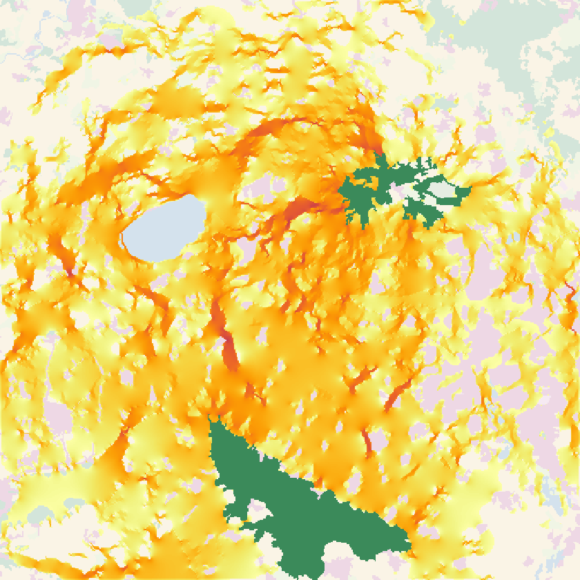


What the slider shows:
- The random walk goes everywhere. Its passages cover the whole landscape thinly: no cell outside the forests sees more than 3% of the walkers, and the brightest channels are the woods and pastures that conduct best, wherever they are. Up to the connection scheme, it is Circuitscape's current between the two forests (Circuitscape).
- Small θ draws a broad band. At θ = 0.0001 the walkers keep to the half of the landscape between the forests, in a band some 15 km wide, with denser channels inside it.
- Large θ draws the corridor. From θ = 0.001 the band narrows; at θ = 0.01, 72% of the walkers pass through the busiest cell, and the passages trace the least-cost corridor of part 1.
- The robust corridor. The channel north through the centre-west and east past the lake is bright at every θ from 0.0001 up: the strongest evidence for a corridor is that it survives the choice of the movement model.
The count of cells with passage of at least 0.01 first grows (walkers concentrate from everywhere into the band) then shrinks (the band narrows to a corridor); the peak passage only grows.
Distances: random walk, RSP and least cost#
At θ = 0.00001 an RSP walker spends on average 6,957 (cells of forest) to go from the southern forest to the north-eastern one, three times the least cost (2,189); at θ = 0.01, 3,126, still 43% above it. The expected cost is the price of not knowing the way, and it falls as walkers know more.
Between the five forests, the three distances rank the ten pairs almost alike: the rank correlation of least costs with commute distances is 0.95, with RSP distances (θ = 0.0001 or 0.003) 0.98. The pairs are far enough apart, and the landscape's main corridors clear enough, that the models agree on which forests are isolated; they disagree on how walkers get between them. That is the general lesson: distances are robust to the movement model, maps of movement much less.
| Pair of forests | Least cost (cells) | Commute distance (millions) |
|---|---|---|
| North-east – Far north-east | 611 | 1.64 |
| North-east – North-west | 752 | 2.21 |
| South – South-west | 1,023 | 1.78 |
| North-west – Far north-east | 1,320 | 2.72 |
| South-west – North-west | 1,566 | 2.79 |
| South – North-west | 1,924 | 2.68 |
| South – North-east | 2,189 | 3.01 |
| North-east – South-west | 2,308 | 3.41 |
| South – Far north-east | 2,795 | 3.53 |
| South-west – Far north-east | 2,876 | 3.94 |
The commute distance is large (a walker going from one forest to another and back takes millions of cost units of wandering) and compressed: the closest pair is at 42% of the farthest, against 21% for least costs. Random walkers waste so much on wandering that distance matters relatively less to them.
In the literature
Report the resistance, the transition and its correction, the origins and goals, and θ with its cost units; better, show results at several θ, as above. Panzacchi et al. (2016) chose θ by fitting it to observed movements; without movement data, present a range. van Etten (2017) documents the gdistance functions these operators reproduce.
Settings that change the answer#
- θ, as above, relative to the cost units. Rescale the costs (
scale) and θ changes meaning. - The correction:
cfor costs and RSP,rfor random walks; usingcfor a random walk changes the passages at the cells' edges. total_net: net passages (the default) count a back-and-forth as nothing; total passages count both crossings, and are larger where walkers hesitate.gdistance_compat(random walks): gdistance's convention for the grounded cell (the default) or the exact currents (false); the difference is visible only next to the goal.- The resistance, as for every model of the series.
Common pitfalls#
- θ copied from another study. θ depends on the cost units and on the resistance's scale. A θ of 0.05 from the template (costs in cells of a 100 × 100 grid) means something else on another map.
- Too large θ. Above some value the walkers all take the least-cost path and nothing more is learned; θ is limited to 20, and useful values are usually far smaller.
- Passages read as probabilities of use. They are net crossings per walker from origin to goal; a cell with passage 0.3 is crossed (net) by three walkers in ten.
- Random walks on uncorrected transitions. Without the geographic correction, diagonal steps are as likely as side steps, and the walk drifts diagonally.
Going further#
- Part 1: cost distance, paths and corridors.
- Circuit theory: the random walk as electric current.
- Habitat networks: habitat graphs with least-cost and
commute-time distances (
distance = "commute-time"), andconn.graph_from_samcfor settling probabilities of absorbing random walks. - The operators:
cost.passage,cost.rsp_distance,cost.commute_distance,cost.path_inc,cost.normalize,cost.barriers,cost.areas,cost.mahal.
References#
- Chandra, A. K., Raghavan, P., Ruzzo, W. L., Smolensky, R., & Tiwari, P. (1996). The electrical resistance of a graph captures its commute and cover times. Computational Complexity, 6(4), 312–340. https://doi.org/10.1007/BF01270385
- Doyle, P. G., & Snell, J. L. (1984). Random walks and electric networks. Mathematical Association of America. https://doi.org/10.5948/UPO9781614440222
- Kivimäki, I., Shimbo, M., & Saerens, M. (2014). Developments in the theory of randomized shortest paths with a comparison of graph node distances. Physica A: Statistical Mechanics and its Applications, 393, 600–616. https://doi.org/10.1016/j.physa.2013.09.016
- McRae, B. H. (2006). Isolation by resistance. Evolution, 60(8), 1551–1561. https://doi.org/10.1111/j.0014-3820.2006.tb00500.x
- McRae, B. H., Dickson, B. G., Keitt, T. H., & Shah, V. B. (2008). Using circuit theory to model connectivity in ecology, evolution, and conservation. Ecology, 89(10), 2712–2724. https://doi.org/10.1890/07-1861.1
- Panzacchi, M., Van Moorter, B., Strand, O., Saerens, M., Kivimäki, I., St. Clair, C. C., Herfindal, I., & Boitani, L. (2016). Predicting the continuum between corridors and barriers to animal movements using Step Selection Functions and Randomized Shortest Paths. Journal of Animal Ecology, 85(1), 32–42. https://doi.org/10.1111/1365-2656.12386
- Saerens, M., Achbany, Y., Fouss, F., & Yen, L. (2009). Randomized shortest-path problems: two related models. Neural Computation, 21(8), 2363–2404. https://doi.org/10.1162/neco.2009.11-07-643
- van Etten, J. (2017). R package gdistance: distances and routes on geographical grids. Journal of Statistical Software, 76(13). https://doi.org/10.18637/jss.v076.i13
- van Etten, J., & Hijmans, R. J. (2010). A geospatial modelling approach integrating archaeobotany and genetics to trace the origin and dispersal of domesticated plants. PLoS ONE, 5(8), e12060. https://doi.org/10.1371/journal.pone.0012060