Sediment delivery ratio

Rain loosens soil on bare and grazed slopes, and part of it ends up in the rivers, where it clouds the water, smothers the gravel fish spawn in and fills reservoirs. Vegetation holds the soil, and strips of forest between a field and a stream trap what still comes down: an ecosystem service with a price, since dredging a reservoir is expensive. InVEST's sediment delivery ratio (SDR) model maps both halves of the story: how much soil each cell loses, and how much of it reaches a stream. In this tutorial you will build it in Terraflux on Ribeirão Claro, read its maps of soil loss, connectivity, export, deposition and retention, find out which settings it is sensitive to, see what roads that drain to the streams do, and compare the scenario of 2040 with 2020.

The idea#

The model chains two classic ideas.

How much soil a cell loses. The Universal Soil Loss Equation (USLE), built in the United States from decades of measurements on erosion plots and revised as the RUSLE (Renard et al., 1997), predicts the average annual loss from sheet and rill erosion (the thin film and small channels of water running over the surface) as a product of five factors.

Key idea: the soil loss of the RUSLE

\[ \text{USLE}_x = R_x \cdot K_x \cdot LS_x \cdot C_j \cdot P_j \quad (\text{t / ha / yr}) \]

\(R\), the rainfall erosivity (MJ mm / (ha h yr)): how hard and how intensely it rains;
\(K\), the soil erodibility (t ha h / (ha MJ mm)): how easily the soil detaches, from its texture and organic matter;
\(LS\), the slope length and steepness factor: steeper and longer slopes lose more. InVEST computes it from the elevation model and the area draining into each cell, in the form of Desmet and Govers (1996) for complex terrain; the slope length factor \(L\) is capped at l_max (122 by default);
\(C\), the cover-management factor of the land use class (0 to 1): 1 for bare soil, near 0 under dense forest;
\(P\), the support practice factor (0 to 1): contour farming, terraces, strips (1 without any).

\(R \cdot K \cdot LS\) alone (the output rkls) is the loss of the cell if it were bare; the difference \(\text{RKLS} - \text{USLE}\) (avoided_erosion) is the erosion its vegetation and practices prevent.

How much of it reaches a stream. Most eroded soil is deposited again on the way down: at the foot of the slope, in a hedge, in a strip of forest. Borselli et al. (2008) proposed an index of connectivity (IC) that measures how well a cell is linked to the stream below it, from two parts: what comes from upslope (a large, steep, bare area makes a cell well connected) and the path down (a long, gentle, vegetated path makes it poorly connected). Vigiak et al. (2012) turned the index into a sediment delivery ratio with a sigmoid curve, and Hamel et al. (2015) built the two into InVEST.

Key idea: connectivity and delivery

\[ IC_x = \log_{10}\frac{D_{\text{up}}}{D_{\text{dn}}}, \qquad D_{\text{up}} = \bar{C}\,\bar{S}\,\sqrt{A}, \qquad D_{\text{dn}} = \sum_i \frac{d_i}{C_i\,S_i} \]

where \(A\) is the area draining into the cell (m²), \(\bar{C}\) and \(\bar{S}\) the mean cover factor and slope (m/m) of that area, and the sum runs over the cells \(i\) of the path from the cell to the stream, \(d_i\) being the length of the path through cell \(i\). (Slopes are kept between 0.005 and 1 and \(C\) above 0.001, as Cavalli et al. (2013) and InVEST do, so that no term is zero.) Then

\[ SDR_x = \frac{SDR_{\max}}{1 + \exp\left(\dfrac{IC_0 - IC_x}{k}\right)} \]

with \(SDR_{\max}\) the largest share that can be delivered (0.8 by default), \(IC_0\) the index at which half of that is delivered (0.5), and \(k\) the steepness of the curve (2). The sediment export of the cell is \(\text{USLE}_x \cdot SDR_x\); stream cells have SDR 1.

A worked cell: pasture on a slope with \(R = 5\,500\), \(K = 0.03\), \(LS = 5\), \(C = 0.05\), \(P = 1\) loses \(5\,500 \times 0.03 \times 5 \times 0.05 = 41\) t / ha / yr; bare, it would lose \(825\). If its index of connectivity is \(-3\) (a typical hillslope value here), its SDR is \(0.8 / (1 + e^{(0.5 + 3)/2}) = 0.12\): 4.9 t / ha / yr reach the stream, the rest is deposited downslope. At \(IC = -6\), farther from the stream behind forest, the SDR falls to 0.03.

The sediment delivery ratio against the index of connectivity — Vigiak's sigmoid with InVEST's defaults (SDR_max 0.8, IC_0 0.5) for four values of k. A larger k flattens the curve and delivers more sediment from poorly connected cells, whose indices are far below IC_0.

The sediment that does not reach a stream is deposited on the cells below, which then retain it: the model routes it down the flow paths (sed_deposition) and counts as avoided export (avoided_export) both the erosion the vegetation prevents (times its SDR) and the sediment the cell traps from upslope.

When to use it#

Where to restore: the cells whose vegetation keeps the most sediment out of the rivers, or would if restored (riparian strips, steep pasture).
Scenarios: how much more sediment a reservoir receives if pasture replaces forest, or less if farmers adopt practices that lower \(P\).
Payments for watershed services and water funds, targeting the farms upstream of an intake.

What it is not: the RUSLE covers sheet and rill erosion only. Gullies, landslides, river banks and construction sites, often the largest sources of sediment, are not in the model. Its numbers are averages of many years. Uncalibrated, the export can differ from measured loads by a large factor; calibrate \(k\) (below) against the sediment measured at a gauge or in a reservoir, and use the model to compare scenarios. Hamel et al. (2015), testing it on eight sub-catchments of the Cape Fear basin (North Carolina), found that the export depended most on the erosivity, the erodibility and the cover factor of farmland; the model ranked the sub-catchments well and its exports were highly correlated with the observed ones, but they warned that absolute values need local knowledge of the dominant erosion processes before they inform decisions.

What you need#

Input	File	Unit
`dem`	`dem.tif`	m, projected; the model fills its depressions and routes the flow over it
`erosivity`	`erosivity.tif`	\(R\), MJ mm / (ha h yr)
`erodibility`	`erodibility.tif`	\(K\), t ha h / (ha MJ mm)
`lulc`	`lulc_2020.tif`	class codes
`biophysical`	`biophysical_sdr.csv`	by class: `lucode`, `usle_c`, `usle_p`
`watersheds`	`watersheds.gpkg`	polygons (with `ws_id`, else numbered 1, 2...): the model runs inside them
`drainage` (optional)	`roads_2020.tif`	1 where the land drains to a stream otherwise (roads, ditches)

The biophysical table here (illustrative values; use local or regional tables of the RUSLE's \(C\) and \(P\)):

lucode	class	usle_c	usle_p
1	Forest	0.001	1
2	Pasture	0.05	1
3	Cropland	0.2	0.5
4	Eucalyptus	0.03	1
5	Urban	0.01	1
6	Water	0	1

Cropland has the highest \(C\) but \(P = 0.5\): its farmers plough along the contours.

Build the model#

Add raster.read nodes for dem.tif, erosivity.tif, erodibility.tif and lulc_2020.tif, a table.read for biophysical_sdr.csv and a vector.read for watersheds.gpkg.
Add services.sdr (subject Ecosystem services) and connect each to the input of its name.
Set threshold, the number of cells that must drain into a cell for it to be a stream. Here 1,000 cells (90 ha) draws the main rivers and their larger tributaries; see below how to choose it. Leave k, ic_0, sdr_max, l_max and method at InVEST's defaults (2, 0.5, 0.8, 122, mfd).
Run (Ctrl+Enter).

The sediment delivery ratio model of 2020.

Model file (TOML)

format = "terraflux/1"

[[nodes]]
id = "dem"
op = "raster.read"
params = { path = "dem.tif" }

[[nodes]]
id = "erosivity"
op = "raster.read"
params = { path = "erosivity.tif" }

[[nodes]]
id = "erodibility"
op = "raster.read"
params = { path = "erodibility.tif" }

[[nodes]]
id = "lulc"
op = "raster.read"
params = { path = "lulc_2020.tif" }

[[nodes]]
id = "biophysical"
op = "table.read"
params = { path = "biophysical_sdr.csv" }
note = "lucode, usle_c, usle_p."

[[nodes]]
id = "watersheds"
op = "vector.read"
params = { path = "watersheds.gpkg" }

[[nodes]]
id = "sediment"
op = "services.sdr"
inputs = { dem = "dem.raster", erosivity = "erosivity.raster", erodibility = "erodibility.raster", lulc = "lulc.raster", biophysical = "biophysical.table", watersheds = "watersheds.vector" }
params = { threshold = 1000, k = 2, ic_0 = 0.5, sdr_max = 0.8, l_max = 122, method = "mfd" }

Behind the node, the chain is InVEST's: the DEM's depressions filled, the flow routed by multiple flow directions (mfd: each cell's water split among its lower neighbours, as pygeoprocessing does) or by d8 (all of it to the steepest neighbour), the flow accumulated, the streams traced, the slope, the LS factor, the connectivity, the SDR and the deposition. Its outputs:

Output	What it is	Unit
`rkls`	soil loss of bare soil, \(R\,K\,LS\)	t / ha / yr
`usle`	soil loss with the land use, \(R\,K\,LS\,C\,P\)	t / ha / yr
`ic`, `sdr`	index of connectivity, sediment delivery ratio
`sed_export`	soil loss that reaches a stream, USLE × SDR	t / ha / yr
`sed_deposition`	sediment from upslope that the cell traps	t / ha / yr
`avoided_erosion`	RKLS − USLE	t / ha / yr
`avoided_export`	avoided erosion × SDR + deposition	t / ha / yr
`stream`, `drains_to_stream`	the streams (1); 1 where the flow reaches one
`watershed_table`	by watershed: `usle_tot`, `sed_export`, `sed_dep`, `avoid_exp`, `avoid_eros`	t / yr

Stream cells have no soil loss (the RUSLE is for hillslopes), and cells outside the watersheds are left out. Only the index of connectivity is wanted? hydro.connectivity_index computes it alone, from a DEM and a weight (usually the \(C\) factor).

Read the results#

Soil loss and connectivity#

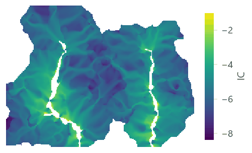
Export, deposition and retention#

sed_deposition, t / ha / yr — sed_export, t / ha / yr

Watershed	Soil loss	Export	Deposition	Avoided export	Avoided erosion
1	20,176	1,046	19,149	57,517	1,019,235
2	16,612	875	15,718	43,249	658,563

The output watershed_table, tons per year. Of the 20,176 t of soil watershed 1 loses each year, 1,046 t (5%) reach the streams and the rest is deposited on the way down. The vegetation avoids the erosion of over a million tons.

The soil loss splits exactly into export and deposition: \(1\,046 + 19\,149 = 20\,176\) t in watershed 1. Which classes send the sediment?

Class	Mean soil loss (t / ha / yr)	Mean SDR	Mean export (t / ha / yr)	Export (t / yr)
Forest	0.88	0.038	0.034	41.3
Pasture	23.14	0.053	1.247	1,447.2
Cropland	15.85	0.048	0.771	396
Eucalyptus	12.49	0.045	0.619	32
Urban	5.29	0.059	0.352	4.9
Water	0	0.062	0	0

Soil loss, delivery and export by class in 2020. Pasture, on steep slopes with little protection, sends three quarters of the sediment; cropland loses less per hectare because it lies on gentler ground and is farmed along the contours (P = 0.5).

Reporting a sediment analysis

Report the sources of \(R\), \(K\) and the DEM (with its resolution), the \(C\) and \(P\) table, the threshold, \(k\), \(IC_0\), \(SDR_{\max}\), \(l_{\max}\) and the routing, and how you calibrated them. Give the export of each watershed for each scenario, and the avoided export as the measure of the service.

Roads that drain to the streams#

Roads, ditches and storm water pipes carry runoff straight to the streams: InVEST's drainage input marks such cells, where the routing stops and the sediment is taken to reach the stream. Connect a map of them to the input drainage (1 where the land drains to a stream, here roads_2020.tif):

The roads made drainage: their cells count as stream ends for the connectivity.

Model file (TOML)

format = "terraflux/1"

[[nodes]]
id = "roads"
op = "raster.read"
params = { path = "roads_2020.tif" }

[[nodes]]
id = "sediment"
op = "services.sdr"
inputs = { dem = "dem.raster", erosivity = "erosivity.raster", erodibility = "erodibility.raster", lulc = "lulc.raster", biophysical = "biophysical.table", watersheds = "watersheds.vector", drainage = "roads.raster" }
params = { threshold = 1000 }

More export with roads that drain to the streams — The export with the roads draining to the streams minus without them: the slopes just above the roads, now better connected, send more sediment. The landscape's export rises from 1,921 to 2,099 t / yr (+9%).

The scenario of 2040#

Change of export from 2020 to 2040 — The change of sediment export (t / ha / yr): more where forest became pasture or cropland on steep ground (orange); less on the restored riparian strips and on the slopes above them (purple), because the forest of the strips, with its low C factor, raises the downslope part (D_dn) of their index of connectivity.

Quantity (both watersheds)	2020	2040	Change
Soil loss (t / yr)	36,789	60,089	+63.3%
Sediment export (t / yr)	1,921	2,686	+39.8%
Deposition (t / yr)	34,867	57,404	+64.6%
Avoided export (t / yr)	100,766	114,111	+13.2%
Avoided erosion (t / yr)	1,677,798	1,654,498	-1.4%

The two watersheds in 2020 and 2040. Soil loss rises by 63% and export by 40%: the riparian restoration traps part of the extra sediment, so export grows less than soil loss.

Settings that change the answer#

Borselli's k#

InVEST's guide (Natural Capital Alliance, 2026) warns that the model is very sensitive to \(k\) and \(IC_0\), which are not physically based, and, after Vigiak et al. (2012), recommends keeping the defaults (\(IC_0 = 0.5\), \(k = 2\)) and using only \(k\) for calibration (\(SDR_{\max}\) only in advanced studies). In Ribeirão Claro its effect is enormous, because most hillslope cells have indices far below \(IC_0\), on the flat lower part of the sigmoid:

The sediment export of the two watersheds for k from 0.5 to 4: from 4 t / yr to 6,002 t / yr. The soil loss does not change with k; what is not exported is deposited.

A factor of three between \(k = 1.5\) and \(k = 3\): without a measured load to calibrate against, the absolute export is poorly known, and only comparisons made with the same \(k\) are reliable.

The stream threshold#

The threshold decides where hillslopes end and streams begin. A smaller threshold draws more streams, so every cell is closer to one and better connected:

Stream threshold (cells) 250 — Sediment export (logarithmic scale) and the streams (blue) for thresholds from 250 to 4,000 cells (22 to 360 ha). More streams reach into the hills and the export rises: from 1,380 t / yr with the largest threshold to 2,636 t / yr with the smallest.

Stream threshold (cells) 500 — Sediment export (logarithmic scale) and the streams (blue) for thresholds from 250 to 4,000 cells (22 to 360 ha). More streams reach into the hills and the export rises: from 1,380 t / yr with the largest threshold to 2,636 t / yr with the smallest.

Choose the threshold so that the streams match a map of the real rivers (or what you see on imagery), not to reach a number.

Multiple flow directions or D8#

mfd — The SDR with multiple flow directions (left, the default) and with D8 (right), same colour scale (0 to 0.8). D8 sends each cell's water down a single path, so the paths are narrower and the connectivity patchier; the export of the landscape rises from 1,921 to 2,423 t / yr.

The SDR with multiple flow directions (left, the default) and with D8 (right), same colour scale (0 to 0.8). D8 sends each cell's water down a single path, so the paths are narrower and the connectivity patchier; the export of the landscape rises from 1,921 to 2,423 t / yr.

Routing	Export (t / yr)	Deposition (t / yr)
mfd	1,921	34,867
d8	2,423	33,214
mfd, roads drain to the streams	2,099	34,365

Export and deposition of the two watersheds with each routing, and with the roads as drainage.

Common pitfalls#

Units of R and K. Erosivity and erodibility come in US customary units in older sources; InVEST's are SI (MJ mm / (ha h yr) and t ha h / (ha MJ mm)). The conversion factors are 17.02 for \(R\) and 0.1317 for \(K\); a mistake makes the soil loss wrong by those factors.
The DEM's resolution. LS and the connectivity come from the DEM: a 90 m DEM gives other slopes, other paths and another export than a 30 m one. Use the finest DEM that is reliable, and the same for every scenario.
Watersheds that cut the flow. The model runs only inside the watersheds; a polygon that does not follow the divides cuts flow paths and changes the connectivity near its edge. Delineate them from the same DEM (hydro.watersheds).
Sinks. The model fills the DEM's depressions; a real lake or a karst sink becomes a flat it routes across.
Reading the export as the load at the outlet. In-stream processes (deposition in the channel, bank erosion) are not modelled.
Forgetting the threshold. It changes the streams, the SDR (1 on streams) and which cells have a soil loss.

Going further#

Ecosystem service models: the ideas for the series' models together.
Nutrient delivery ratio, the next part: nitrogen and phosphorus on the same connectivity.
Annual water yield on the same watersheds.
Terrain from an elevation model for slopes and the shape of the land.
The operators' reference: services.sdr, hydro.connectivity_index, hydro.watersheds.

References#

Borselli, L., Cassi, P., & Torri, D. (2008). Prolegomena to sediment and flow connectivity in the landscape: A GIS and field numerical assessment. Catena, 75(3), 268–277. https://doi.org/10.1016/j.catena.2008.07.006
Cavalli, M., Trevisani, S., Comiti, F., & Marchi, L. (2013). Geomorphometric assessment of spatial sediment connectivity in small Alpine catchments. Geomorphology, 188, 31–41. https://doi.org/10.1016/j.geomorph.2012.05.007
Desmet, P. J. J., & Govers, G. (1996). A GIS procedure for automatically calculating the USLE LS factor on topographically complex landscape units. Journal of Soil and Water Conservation, 51(5), 427–433. https://doi.org/10.1080/00224561.1996.12457102
Hamel, P., Chaplin-Kramer, R., Sim, S., & Mueller, C. (2015). A new approach to modeling the sediment retention service (InVEST 3.0): Case study of the Cape Fear catchment, North Carolina, USA. Science of the Total Environment, 524–525, 166–177. https://doi.org/10.1016/j.scitotenv.2015.04.027
Natural Capital Alliance. (2026). InVEST 3.20.2 User's Guide: SDR, sediment delivery ratio. https://storage.googleapis.com/releases.naturalcapitalproject.org/invest-userguide/latest/en/sdr.html
Renard, K. G., Foster, G. R., Weesies, G. A., McCool, D. K., & Yoder, D. C. (1997). Predicting Soil Erosion by Water: A Guide to Conservation Planning With the Revised Universal Soil Loss Equation (RUSLE) (Agriculture Handbook No. 703). U.S. Department of Agriculture.
Vigiak, O., Borselli, L., Newham, L. T. H., McInnes, J., & Roberts, A. M. (2012). Comparison of conceptual landscape metrics to define hillslope-scale sediment delivery ratio. Geomorphology, 138(1), 74–88. https://doi.org/10.1016/j.geomorph.2011.08.026