PLUS: land expansion and random patch seeds

In this tutorial you simulate the growth of built land on the coast of Massachusetts, around the Plum Island estuary, with PLUS, one of the most used land change models of the last few years. You will learn where each land use expanded between 1985 and 1991 with a random forest, project the areas with a Markov chain, and let PLUS's cellular automaton (CARS) place the change from 1991 to 1999, growing existing patches and planting new ones. At the end you will compare the simulation with the map actually observed in 1999 and see why the answer depends on the scale at which you look.

The idea#

PLUS, the patch-generating land use simulation model (Liang et al., 2021), is made of two parts.

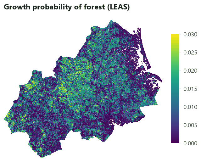
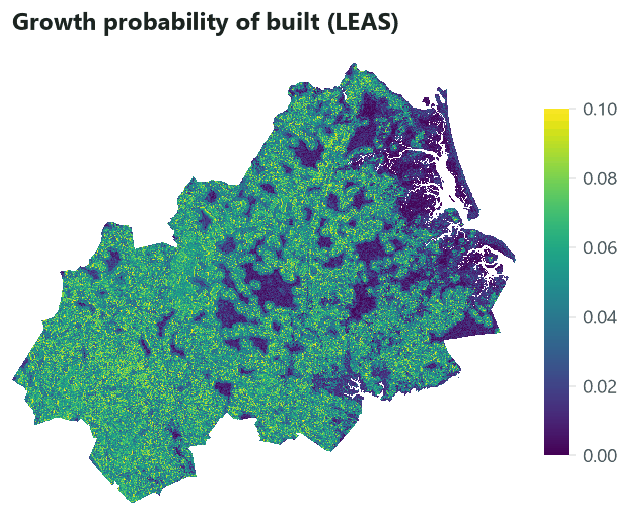
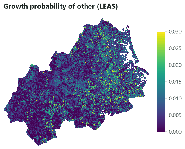
LEAS, the land expansion analysis strategy. To know where a land use is likely to appear, most models fit their suitability on where the land use is (as CLUE-S does). But the places where cities already stand mix old and new land uses: the centre of a town tells little about where it grows today. LEAS fits the model only on the cells that changed: it compares two maps, keeps the cells that gained each class (the expansion), and trains a random forest for each class to separate those cells from the others. A random forest (Breiman, 2001) is a set of decision trees, each trained on a random sample of the cells and of the drivers; their votes give a probability. Its output, for each class, is a map of the growth probability, and its by-product is the contribution of each driver (the importance of the variable in the forest).

CARS, the CA based on multi-type random patch seeds. A cellular automaton (CA) is a grid whose cells change state by rules that look at their neighbours. CARS repeats iterations until every class has the number of cells the demand asks for. In each iteration, every cell gives every class an overall probability made of three parts: its growth probability (from LEAS), the share of its neighbours that already have the class, and an adaptive coefficient that rises while the class falls short of its demand. A roulette wheel picks a class from these probabilities, and the cell changes if its growth probability for that class passes a threshold that decreases over the iterations. Where no neighbour has the class, a random seed can still start a new patch: this is what lets PLUS create new settlements away from the old ones, and what gives it its name.

The decaying threshold makes the cells of highest growth probability change first: at the start only the very best cells pass \(\tau \approx 1\); as the iterations fail to close the gap, \(\tau\) falls and more cells qualify. The neighbourhood term makes change cling to existing patches; the random seeds, weighted by \(\mu_k\), let new patches appear.

When to use it#

PLUS is a good choice when:

• several classes change at once and compete for the same land (cropland, built land, forest, water);
• new patches matter, not only the growth of existing ones (new settlements, new plantations);
• you want to know which drivers explain the expansion of each class (the random forest's contributions);
• you run scenarios of demand (trend, ecological protection, economic development), as in the many studies of Chinese cities and basins that use it (for example Gao et al., 2022, in Nanjing).

It is less suited when the demand is in goods and services rather than areas (CLUMondo), when the patches must reproduce a measured size distribution (Dinamica EGO's Expander and Patcher, or FUTURES), or when you have few cells of change to learn from: a random forest on a few hundred cells overfits. With a single transition (forest to pasture) and a demand in areas, CLUE-S is simpler. See Choosing a model.

What you need#

• Two maps of land use of the same grid for the calibration period, and the map to start from. Here lulcc's example data of the Plum Island Ecosystems (Moulds et al., 2015): pie_landuse.tif, three bands named 1985, 1991 and 1999, 497 by 434 cells of 100 m, with 1 forest, 2 built, 3 other.
• Drivers on the same grid: pie_drivers.tif with elevation, slope and dist_built_1985 (the distance to built land in 1985).
• The growth probabilities of LEAS: a raster with a band per class, named by the class (1, 2, 3). Terraflux has no random forest operator; the probabilities are made with landschaft (below) or any other tool, and read with raster.read.

Enlarge

Build the model#

1. LEAS: the growth probabilities#

LEAS needs a classifier, which Terraflux does not have. landschaft's Estimator with target="expansion" does what LEAS does: for each class, the cells that gained it between the two maps are the presences, the cells that could have gained it and did not are the absences; a sample of both (5 % of the cells, drawn from each group separately, as in the paper) trains a random forest of 50 trees.

import landschaft as ls
import numpy as np, rasterio
from sklearn.ensemble import RandomForestClassifier

S = ls.simulate
lu = ls.load_raster("pie_landuse.tif")
ef = ls.load_raster("pie_drivers.tif")
t0, t1 = lu[0].where(lu[0] != 255), lu[1].where(lu[1] != 255)      # 1985, 1991

leas = S.Estimator(RandomForestClassifier(n_estimators=50, min_samples_leaf=50, random_state=1),
                   target="expansion", classes=[1, 2, 3], sample=0.05, stratify=True, seed=1)
leas.fit(t0, ef, t1=t1)
print(leas.importance())                      # the contribution of each driver to each class
p = leas.predict(ef, landscape=t1)            # a layer per class: the growth probability
# ... written to potential.tif, a band per class named "1", "2", "3"

min_samples_leaf=50 keeps each leaf of the trees above 50 cells, which smooths the probabilities: with leaves of single cells, a forest memorises its training cells and its map of probabilities becomes noisy. landschaft's presets.plus does all of this and the Markov chain in one call, and Model.save writes the result as a Terraflux graph.

2. The probabilities and the demand in Terraflux#

The model reads the start (1991) and the growth probabilities. stack.classes turns the bands named 1, 2, 3 into a stack whose layers are the classes, which is what cars.step looks up.

The demand of PLUS is by default a Markov chain: markov.fit measures the share of each class that went to each other class between 1985 and 1991 and, with steps = 6, the yearly rates (the sixth root of the matrix). plus.demand projects them from the map of 1991 for steps = 8 years and rounds them to whole cells that add up to the map's: the number of cells each class must have at each step. It could take an area demand instead (demand, from demand.table), for a scenario written by hand.

format = "terraflux/1"

[[nodes]]
id = "lu1985"
op = "raster.read"
params = { path = "pie_landuse.tif", band = "1985" }

[[nodes]]
id = "lu1991"
op = "raster.read"
params = { path = "pie_landuse.tif", band = "1991" }
note = "The start."

[[nodes]]
id = "leas"
op = "raster.read"
params = { path = "potential.tif" }
note = "LEAS's growth probabilities, a band per class."

[[nodes]]
id = "growth"
op = "stack.classes"
inputs = { stack = "leas.raster" }

[[nodes]]
id = "markov"
op = "markov.fit"
inputs = { t0 = "lu1985.raster", t1 = "lu1991.raster", steps = 6 }
note = "Yearly rates of 1985-1991."

[[nodes]]
id = "demand"
op = "plus.demand"
inputs = { start = "lu1991.raster", markov = "markov.markov" }
params = { steps = 8 }
note = "The cells of each class, 1992 to 1999."

3. The loop: one CARS step per year#

control.repeat runs cars.step once per year. Its times is demand.steps (8), so the loop follows the demand. The map is the only value carried: @landscape starts as the map of 1991 and takes cars.landscape after each year. cars.step reads the demand of the year from its step input (@step), so it must be connected; and seed gives the random numbers.

format = "terraflux/1"

[[nodes]]
id = "lu1985"
op = "raster.read"
params = { path = "pie_landuse.tif", band = "1985" }

[[nodes]]
id = "lu1991"
op = "raster.read"
params = { path = "pie_landuse.tif", band = "1991" }

[[nodes]]
id = "leas"
op = "raster.read"
params = { path = "potential.tif" }

[[nodes]]
id = "growth"
op = "stack.classes"
inputs = { stack = "leas.raster" }

[[nodes]]
id = "markov"
op = "markov.fit"
inputs = { t0 = "lu1985.raster", t1 = "lu1991.raster", steps = 6 }

[[nodes]]
id = "demand"
op = "plus.demand"
inputs = { start = "lu1991.raster", markov = "markov.markov" }
params = { steps = 8 }

[[nodes]]
id = "simulation"
op = "control.repeat"
inputs = { times = "demand.steps", landscape = "lu1991.raster" }
note = "A step per year of the demand; the map carried."

[nodes.body]
carry = { landscape = "cars.landscape" }
collect = { maps = "cars.landscape", info = "cars.info" }

[[nodes.body.nodes]]
id = "cars"
op = "cars.step"
inputs = { landscape = "@landscape", probability = "growth.stack", demand = "demand.demand", step = "@step", seed = 1 }
params = { seeds = 0.1, weights = { 1 = 0.5, 2 = 1.0, 3 = 0.3 }, decay = 0.9, step_size = 50, window = 3, max_iter = 5000 }
note = "PLUS's CA of multi-type random patch seeds."

The settings of cars.step, with their meaning:

A restrictions input keeps the cells it marks (non-zero) as they are: a protected area, water.

In the application, cars.step and plus.demand are in the Land change simulation subject, group PLUS. Build the loop as in the other tutorials: add control.repeat (Model flow) and, in its Node pane, give it times (demand.steps) and an input named like the carried value, landscape (lu1991.raster). Double-click the loop (or Open inside in the Node pane) to go inside its body: the column on the left lists what the body can read, @landscape, @step and the outer nodes. Add cars.step and connect @landscape, @step and the outer growth.stack and demand.demand. Then go back up (‹ Back, or Esc on the canvas), select the loop, and in its Node pane's Body section choose carry, type landscape and cars.landscape and click Set; choose collect and do the same for maps (cars.landscape) and info (cars.info).

4. Compare with 1999#

To judge the simulation, compare its last map with the map observed in 1999, from the same start. The output of the loop named like the carried value, simulation.landscape, is the map after the last step. validate.three_map compares three maps (the start, the observed end and the simulated end) and gives the figure of merit: the cells where the change was simulated right, divided by all the cells where change was observed or simulated (Pontius et al., 2008). With factors it does so again on blocks of 2, 4, 8 and 16 cells, to see how near the simulated change is to the observed one.

[[nodes]]
id = "lu1999"
op = "raster.read"
params = { path = "pie_landuse.tif", band = "1999" }

[[nodes]]
id = "validation"
op = "validate.three_map"
inputs = { t0 = "lu1991.map", t1 = "lu1999.raster", simulated = "simulation.landscape" }
params = { factors = [1, 2, 4, 8, 16] }

Run it with terraflux run plus.toml --out output (about 10 seconds).

Read the results#

Each year of the simulation, shown on a part of the map (the centre of the study area) so that the cells can be seen:

Enlarge

PlayYear

The info table (steps.csv) tells how each year went: about 20 iterations per year, the threshold decayed 8 to 17 times, and the gap to the demand closed (gap = 0, converged = 1). If converged is 0, the map of that year does not meet the demand: raise max_iter, or lower step_size so the threshold decays sooner.

The quantity. The Markov chain of 1985-1991 asked for 44,434 cells of built land in 1999; the map of 1999 has 43,455. Built land grew more slowly in the 1990s than in the late 1980s, so the demand overestimates it by about 1,000 cells. This error belongs to the demand, not to CARS: separate it from the error of allocation when you report (Pontius & Millones, 2011).

The location. Swipe to compare the observed and the simulated 1999 on the same part of the map:

Observed 1999

Simulated 1999

Enlarge

At the cell level the figure of merit is 0.03: of every 100 cells where change was observed or simulated, 3 were simulated right. That sounds dismal, but look at how it grows with the resolution:

The model puts the change in the right neighbourhoods much more often than on the right cells. Two things explain the low value at the cell level. First, the observed change is scattered (the map of hits and misses shows it in single cells), which no model of patches can reproduce cell by cell. Second, the drivers explain little of where land expanded here: the growth probabilities are low everywhere and the random forest's map is nearly flat, so the neighbourhood term decides most of the allocation. Published figures of merit are commonly between 0.1 and 0.3 at the resolution of the data (Pontius et al., 2008); a model below that should be reported at the resolution where it becomes useful.

How to report it. Give the drivers' contributions from LEAS, the demand (and how its error compares with the allocation's), the CARS settings, and the figure of merit at several resolutions, with the number of replicates if you ran several seeds. The validation tutorials on the category page explain these measures in detail.

Settings that change the answer#

The neighbourhood's side, window, decides how far from an existing patch a cell can grow without being a random seed: with window = 3 only the cells touching built land feel its pull; with 9, any cell within four cells does. Watch the number of patches of built land:

Enlarge

Playwindow

The figure of merit barely moves, but the landscape does: from 649 patches of built land (fewer than the 839 of the observed 1999 map, the town consolidated) to 1,503 (twice too many). If the next step of your study is a landscape metric or a connectivity analysis, this is the setting to calibrate: compare the number of patches, their mean size or the edge density of the simulated maps with the observed ones over a past period.

The patch generation threshold seeds changes much less here:

A random seed needs a uniform number below the cell's growth probability, and here the probabilities are at most about 0.11: seeds are rare whatever \(\mu_k\). With a potential that gives some cells high probabilities far from the existing patches (a new road, a planned district), seeds decides whether new settlements appear.

Other settings: decay and step_size control how fast the threshold falls (a slow fall puts the change on the cells of highest probability; a fast one spreads it), and the neighbourhood weights per class balance clinging to patches against following the probabilities.

Common pitfalls#

• Training on presence instead of expansion. A random forest of where built land is learns the old town centre; LEAS learns where it grew. Use target="expansion" (and the two maps of the calibration period).
• Probabilities that are not comparable between classes. CARS compares each class's probability with the same threshold. Classes that rarely expand get low probabilities and change late; that is intended, but a classifier that inflates one class's probabilities (a balanced sample for one class only) biases the competition.
• Static drivers that should move. dist_built_1985 is the distance to the built land of 1985; by 1999 it is out of date. Recompute such drivers inside the loop (Dynamic drivers), or use drivers that do not depend on the map.
• Bands not named by class. stack.classes needs layers named 1, 2, 3... A raster written without band descriptions gives layers named by number, which may not be the classes.
• A demand larger than the land can take. If the allowed conversions or the restrictions leave too few cells, a step never converges: info shows the gap left.
• One run. CARS is stochastic. Run replicates (terraflux submit plus.toml --replicates 20) and report the spread, or the probability of change of each cell.

Going further#

• A demand per region: CARS with a Markov chain per region.
• Dynamic drivers: drivers recomputed from the simulated map.
• CLUE-S and FUTURES: other ways of allocating a demand; Choosing a model.
• The operators: cars.step, plus.demand, markov.fit, stack.classes, validate.three_map.

References#

• Breiman, L. (2001). Random forests. Machine Learning, 45(1), 5–32. https://doi.org/10.1023/A:1010933404324
• Gao, L., Tao, F., Liu, R., Wang, Z., Leng, H., & Zhou, T. (2022). Multi-scenario simulation and ecological risk analysis of land use based on the PLUS model: A case study of Nanjing. Sustainable Cities and Society, 85, 104055. https://doi.org/10.1016/j.scs.2022.104055
• Liang, X., Guan, Q., Clarke, K. C., Liu, S., Wang, B., & Yao, Y. (2021). Understanding the drivers of sustainable land expansion using a patch-generating land use simulation (PLUS) model: A case study in Wuhan, China. Computers, Environment and Urban Systems, 85, 101569. https://doi.org/10.1016/j.compenvurbsys.2020.101569
• Moulds, S., Buytaert, W., & Mijic, A. (2015). An open and extensible framework for spatially explicit land use change modelling: the lulcc R package. Geoscientific Model Development, 8(10), 3215–3229. https://doi.org/10.5194/gmd-8-3215-2015
• Pontius, R. G., Jr., Boersma, W., Castella, J.-C., Clarke, K., de Nijs, T., Dietzel, C., et al. (2008). Comparing the input, output, and validation maps for several models of land change. The Annals of Regional Science, 42(1), 11–37. https://doi.org/10.1007/s00168-007-0138-2
• Pontius, R. G., Jr., & Millones, M. (2011). Death to Kappa: birth of quantity disagreement and allocation disagreement for accuracy assessment. International Journal of Remote Sensing, 32(15), 4407–4429. https://doi.org/10.1080/01431161.2011.552923