

Circuit connectivity, part 4 of 4
Omniscape: connectivity everywhere
Map connectivity across a whole landscape without choosing areas to connect, with Omniscape's moving-window circuits, read the cumulative current, the flow potential and the normalised current, and see how the window's radius changes the channels it finds.
- Level
- Advanced
- Time
- 45 min
- Template
- Circuit connectivity
Circuitscape needs areas to connect: reserves, populations, forests. Often there are none to choose. Species live throughout a landscape in varying densities, and climate change asks how everything can move, not just how reserve A reaches reserve B. Omniscape answers with circuits too, but everywhere at once: it connects every cell to its neighbourhood, and adds up the currents. In this last part of the series you run it on the landscape around Hannover, read its three maps (cumulative current, flow potential and normalised current), and move a slider over the size of the neighbourhood to see which channels appear for species that move 1 to 5 km. At the end you will be able to map omnidirectional connectivity, choose its settings and read where movement is channelled or impeded.
The idea#
Moving-window circuits#
McRae et al. (2016) built Omniscape to map connectivity for the whole Pacific Northwest of the United States, "wall to wall", for the movement of plants and animals under climate change. Its algorithm (Landau et al., 2021, for the Julia version, Omniscape.jl) is a moving window of circuits:
- Every cell (or one cell in every block of
block_size×block_size) is in turn a target, grounded. - Every cell within
radiusof the target is a source, injecting current in proportion to its source strength: by default its conductance (1 / resistance), so good habitat sends more current, as if it held more animals. - The circuit of the window is solved; its currents are added to the cumulative current map.
The cumulative current of a cell is thus the movement through it among all pairs of places within the radius, weighted by how much habitat each holds. No areas are chosen: every place is a source and a destination.
Key idea: flow potential and normalised current
The cumulative current is high both where the landscape channels movement and where there is simply a lot of habitat sending current. To separate the two, Omniscape runs the same windows a second time with a resistance of 1 everywhere: the flow potential, the current there would be if the landscape offered no resistance, with the same sources. The normalised current is their ratio:
Above 1, movement is channelled (more current than an even landscape would carry: a corridor or pinch point); near 1, it flows as freely as it could; below 1, it is impeded (the landscape blocks movement that would otherwise pass).
When to use it#
- Regional connectivity maps without core areas, for planning or for climate adaptation (McRae et al., 2016).
- Many species at once: with resistance from naturalness or human modification rather than from one species, Omniscape maps the connectivity of "nature" as a whole.
- Finding channels and barriers in continuous habitat: the normalised current.
- Changes: the same model before and after a plan, a road, or a climate change (its
condition1andcondition1_futureinputs restrict movement to places of similar climate now and in the future).
Phillips et al. (2021) compared several methods of mapping omnidirectional connectivity, Omniscape among them, and discuss how their maps differ. When the question is about particular areas, use Circuitscape.
What you need#
- A resistance: here the class resistance of part 2, from
clc_100m.tif. - A radius, in cells: the distance over which the species moves in a lifetime or a generation (Omniscape's window should cover the dispersal distance of interest). Here 10 to 50 cells, 1 to 5 km.
- Time. Omniscape solves one circuit per target. With
block_size = 1, a map of 250,000 cells means 250,000 circuits;block_sizemakes one target per block (and spreads its result over the block), dividing the work by its square. The four runs below took about five minutes together. Try the settings on a small extent first: Stop in the application ends the run, but Omniscape cannot stop in the middle of its circuits and goes on in the background until it is done.
Build the model#
circuit.omniscape (library subject Circuit connectivity) takes the resistance and, optionally, a
source map of source strengths. Its outputs are current (the cumulative current), flow_potential and
normalized (given only when the settings of the same names are on: with them off the model still runs, and only
a node connected to the missing map stops, saying so).
Model file (TOML)
format = "terraflux/1"

[[nodes]]
id = "land"
op = "raster.read"
params = { path = "clc_100m.tif" }

[[nodes]]
id = "resistance"
op = "raster.reclassify"
inputs = { map = "land.raster" }
params = { rules = "23 24 25 -> 1\n29 -> 2\n21 26 27 32 35 36 -> 5\n18 20 -> 10\n12 -> 20\n10 11 -> 30\n7 8 9 -> 50\n1 2 3 4 5 6 40 41 -> 100\n* -> 20" }
note = "A resistance per class (part 2)."

[[nodes]]
id = "omniscape"
op = "circuit.omniscape"
inputs = { resistance = "resistance.map" }
params = { radius = 30, block_size = 5, flow_potential = true, normalized_current = true }
note = "Windows of 30 cells (3 km); a target every 5 cells."

[[plots]]
id = "plot"
title = "Normalised current"
layers = [{ from = "omniscape.normalized" }]
The settings:
radius: the window's radius in cells. The most important choice (below).block_size: an odd number of cells; one target per block. 1 is exact; 3 to 9 are usual for large maps.correct_artifacts(on by default) smooths the seams between blocks.source(input) andsource_threshold: your own source strengths (a suitability, a population density) and the value below which a cell sends nothing. Without them, sources are the conductance, andr_cutoffstops cells above a resistance from being sources.buffer: cells beyond the radius included in each window's circuit (but not as sources), so that current can go around obstacles near the window's edge.flow_potential,normalized_current: the two other maps.condition1,condition2(inputs) withcomparison1,condition1_lower,condition1_upper: conditional connectivity, where a source connects to a target only if their conditions (a temperature, an elevation) match within limits.
Omniscape's INI files
circuit.omniscape_ini runs an Omniscape INI file as it is, with every option of Omniscape 0.7, and
writes the outputs as Omniscape names them in its project folder. Use it to repeat an analysis made with
Omniscape.jl, or to share one.
Read the results#
The three maps#
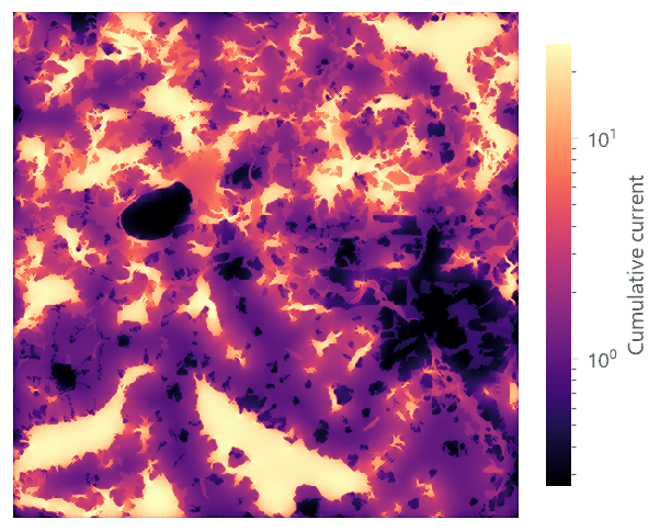

The cumulative current is brightest over the large forests: they are full of strong sources, and current flows freely inside them. It is also bright in strips of woods and pasture between forests, and dark over the lake and Hannover. The flow potential has the same bright forests (it uses the same sources) but none of the landscape's structure. Their ratio is the map to read.
The normalised current at four radii#
Move the slider: each frame is a real run with a different radius (1, 2, 3 and 5 km), coloured with 1 in white, channelled movement in red and impeded movement in blue.


How to read it:
- Inside large forests the normalised current is near 1: movement is as free as it could be, neither channelled nor impeded. Forest is not where connectivity is at stake.
- Red strips are channels: narrow woods, hedges of pasture and heath, and gaps between towns, where movement between forests crowds. These are Omniscape's pinch points, the places to protect, and they multiply with the radius: 1.1% of the landscape is channelled at 1 km, 9.7% at 5 km.
- Blue is impeded: open arable land and towns, where movement that would cross an even landscape goes around. The edges of the large forests are blue at small radii (current leaves them reluctantly into the farmland). The share of impeded land grows from 18% to 25% and then stays.
- The radius sets the question. At 1 km the map describes how animals move around their own wood; at 5 km how they move between forest blocks. Regional plans use the larger radius; a study of a small mammal the smaller.
In the literature
Report the resistance and the source strengths, the radius (in cells and kilometres), the block size, and the
map shown (cumulative or normalised, with its colour scale). McRae et al. (2016) classified the normalised
current into categories (impeded, diffuse, intensified, channelised) to make maps for planners; the same
can be done with raster.reclassify on the normalized output.
From a map to categories for planners#
A continuous ratio is hard to act on. Following McRae et al. (2016), classify the normalised current into a few
categories with one raster.calc on omniscape.normalized:
1 if n < 0.5 else 2 if n < 1.5 else 3 if n < 2.5 else 4
1 impeded (movement blocked, a candidate barrier to remove), 2 diffuse (movement flows as freely as the sources allow), 3 intensified (movement concentrates), 4 channelised (strong pinch points). The thresholds are conventions: state them. In this landscape, at 3 km, a quarter of the land is impeded (mostly arable land far from woods and the towns) and 6% is intensified or channelised.
Model file (TOML)
[[nodes]]
id = "classes"
op = "raster.calc"
inputs = { n = "omniscape.normalized" }
params = { expression = "1 if n < 0.5 else 2 if n < 1.5 else 3 if n < 2.5 else 4" }
note = "1 impeded, 2 diffuse, 3 intensified, 4 channelised."
Omniscape and Circuitscape compared#
The two use the same circuits and differ in what they connect:
| Circuitscape (pairwise) | Omniscape | |
|---|---|---|
| Sources and destinations | chosen focal areas | every cell, within a radius |
| Strength of a source | 1 A per area | the cell's habitat quality (conductance or a source map) |
| Distance limit | none: two areas 50 km apart are connected | the radius |
| Main map | cumulative current between the areas | normalised current |
| Answers | how areas connect, and through where | where the landscape channels or blocks movement in general |
Run on the same resistance, they agree on the main channels between the large forests (compare the pairwise current with the red strips at 5 km), but Omniscape also shows the local channels between small woods that no pair of large forests uses, and the impeded land around every forest edge. A complete connectivity study often uses both: Omniscape for the map of the region, Circuitscape for the links between the areas that matter.
Settings that change the answer#
- The radius, as above. When the dispersal distance is uncertain, run two radii and look for channels present in both.
- The source strengths. Sources from conductance make good habitat the main sender. A separate source map (habitat suitability, or the presence of a species) changes where current starts; a source threshold stops poor habitat from sending at all.
- The block size. Larger blocks are faster but coarser; channels narrower than a block can blur. Check a
small area with
block_size = 1. - The resistance (part 2): as with Circuitscape, the contrasts sharpen or soften the channels.
Common pitfalls#
- Reading the cumulative current as connectivity. It is dominated by where the sources are. Read the normalised current for channels and barriers, and the cumulative current for where most movement goes.
- Edges. Windows near the map's edge are cut, so current there is low and normalised values unreliable. Analyse a buffer of at least the radius around the study area.
- A radius in metres.
radiusis in cells: 30 means 3 km only with cells of 100 m. - Block artefacts. With large blocks and
correct_artifacts = false, a regular pattern of squares appears; keep the correction on. - Run time. Time grows with the square of the radius over the block size. Start small, then refine.
Going further#
- Part 3: Circuitscape, when there are areas to connect.
- Habitat networks: connectivity of habitat patches.
- Grid distances: least costs and random walks.
- The operators:
circuit.omniscape,circuit.omniscape_ini.
References#
- Landau, V. A., Shah, V. B., Anantharaman, R., & Hall, K. R. (2021). Omniscape.jl: software to compute omnidirectional landscape connectivity. Journal of Open Source Software, 6(57), 2829. https://doi.org/10.21105/joss.02829
- McRae, B. H., Popper, K., Jones, A., et al. (2016). Conserving nature's stage: mapping omnidirectional connectivity for resilient terrestrial landscapes in the Pacific Northwest. The Nature Conservancy, Portland, Oregon.
- Phillips, P., Clark, M. M., Baral, S., Koen, E. L., & Bowman, J. (2021). Comparison of methods for estimating omnidirectional landscape connectivity. Landscape Ecology, 36(6), 1647–1661. https://doi.org/10.1007/s10980-021-01254-2