

A tour of Terraflux
The window and its panes, the Templates menu and its groups, opening and running a template, the operators' library and the / search, the viewer, basemaps and the settings, for someone who has never used the application.
- Level
- Beginner
- Time
- 20 min
- Template
- MSPA of a forest
This tutorial is the first thing to read after installing Terraflux. You will open the application, learn the name and the job of every part of its window, open a ready-made model from the Templates menu, run it, look at its map, change one of its settings, and find your way to the hundreds of operators it holds. You need no data of your own and no experience with GIS software: everything here runs on maps that Terraflux draws by itself. At the end you will know where things are, which is all the later tutorials assume.
The idea: an analysis is a chain of boxes#
Most GIS software works through menus: you open a map, choose Raster > Reclassify in a menu, fill a dialog, get a new map, choose the next tool, and so on. When you want to do it again with another map, or with a different setting halfway through, you repeat every click.
Terraflux keeps the chain itself. Each step of an analysis is a node: a box that runs one operator (read a map, reclassify it, compute a fragmentation index...). The boxes are joined by connections that carry a map, a table or a number from the output of one node to the input of the next. The whole chain is a model. Because the model is kept, you can change any step and run it again: Terraflux recomputes only what that change touches. A model is saved as a small text file that you can share, put in the supplementary material of a paper, or run on another computer from the command line.
This way of working is called visual programming or a model builder; ecologists may know it from ArcGIS's ModelBuilder, QGIS's graphical modeler or the land change software Dinamica EGO (Soares-Filho et al., 2002), whose models are drawn the same way.
Key idea
A model is a graph: nodes are operations, connections are the data passed between them. The graph says what depends on what, so the application knows the order to run the nodes in, and which nodes need to run again when you change one.
When to use the application, and when the command line#
Terraflux is two things in one program:
- the application, a window where you build, run and look at models: this tutorial;
- the command line (
terraflux run,terraflux check...), which runs the same model files without a window: for long runs, many runs, servers and clusters. Your first model shows it.
You will usually build and check a model in the application and, when it is right, run it as many times as you need from the command line. Nothing is lost between the two: they read and write the same file.
What you need#
Only Terraflux, installed as the Quickstart explains. The templates used here draw their own maps with neutral landscape models, random maps with a known structure (Gardner et al., 1987; Sciaini et al., 2018), so they run without any file.
The window#
Open Terraflux (from the Start menu on Windows, Applications on macOS, the menu of your desktop on Linux, or by
typing terraflux app in a terminal). The window starts empty, with a message in the middle of the canvas:
Open a raster, click an operator of the library or press / to start; or begin from a template (Templates).

Here is the same window after a template has run, with its parts numbered. The template brings the Node and Prepare panes at the left, and the Document and the Viewer as tabs behind the Model's; here the Viewer's tab was dragged below the Model, to see both:

- The toolbar. The File menu (New model, Open..., Open recent, Save, Save as..., Open a raster or vectors..., Compare and Export report), Templates (models to start from), Operators (the library as a menu) and View (panes on and off); at the right, Wizard... (a land change model built step by step from your maps), Many runs..., Computers..., Assistant... and ⚙, the settings.
- Run and Stop, then the model's name and how long the last run took (done in 0.04 s). Run (F5) runs the whole model. Beside them, Step pauses a run after each step of a loop, until Next or Continue (see Loops).
- The Node pane: the node you selected. Its name (which you can change with Rename), its operator
(
landscape.mspa) and what that operator does, its Inputs (what is connected to it), its Settings, then its record: Note (what the node is for, shown on the canvas), Why (why this operator and these settings), the collapsible References, assumptions, alternatives, and Delete node. With no node selected, the pane holds the model's own record (its name, description, request, summary and author). - The Prepare pane, a tab beside Node: the data of the node selected compared with the model's reference grid, and the steps that put it on that grid in a click (see One grid for all your maps).
- The Model pane: the canvas where the nodes and their connections are drawn. Its tab has the Document tab beside it, the same model read as text (The model's document). A node is as wide as its names need (an input's and an output's never run into each other); drag its right edge to make it wider, and double-click the edge to bring it back to the width its names need.
- The Model pane's bar: where you are in the model (Whole model, or inside a loop), Run to here (run the node selected and what it needs, Ctrl+Enter), Arrange (tidy the nodes, Ctrl+L), Undo and Redo, update after every edit (run again by itself after every change) and Text (the model as text).
- The Viewer. It shows what the node selected gives, refreshed at every run; a double click on a node brings it to the front with that node's output, and keeps it there as a layer. The Layers at the map's left list the maps and vectors drawn together (shown or hidden, dragged over or under each other, their opacity, zoom to see all of one); the Layers button above the map hides them.
- Save output (the map shown as a GeoTIFF file, with or without a
raster.writenode added to the model), the Plots of the model (here Plot: MSPA, the one shown: what the Viewer shows kept with the model, see Plots and figures) and Metadata (what the file or map says about itself: size, cell size, coordinate system, no data...). - The legend: the classes of the map with their colours and their number of cells (here 300 x 300 cells, of which 33,168 are core forest), or a colour bar for continuous values.
- The key hints: a reminder of the mouse and keyboard actions of the pane under the pointer.
Arrange the window your way
Every pane is a tab. Drag a tab to put it beside, above or below another; drag it out of the window and it becomes a window of its own, to put on a second screen (or right-click the tab: Open in a window of its own). Ctrl+W closes the tab in front, and View turns each pane on or off (Many runs, Computers, Simulation, Areas and Validation are off at first). View > Reset the layout brings back the window as it first was. Terraflux remembers the layout between sessions.
Templates: models to start from#
A template is a small, complete model, made to show how a kind of analysis is built. It opens in the Model pane, arranges itself, and runs at once, so you see its result before you have touched anything. Every node of a template has a note that says what it does and what to put in its place for your own study (in its place, a raster.read of a map of yours).
Open the Templates menu. Its templates are in seven groups:

| Group | Its templates | Tutorials |
|---|---|---|
| Patterns (GuidosToolbox) | MSPA of a forest, MSPA of your map, Forest from a surface, Fragmentation of a forest, Patterns and objects, Landscape mosaic, MSPA's edge width, Forest gain and loss | Habitat patterns |
| Landscape metrics | Landscape metrics, Patches and their shapes, Kinds of landscapes | Landscape metrics |
| Connectivity | Network of a forest (MSPA), Habitat network (Conefor), Circuit connectivity, Least costs and random walks, Restoring a corridor | Habitat networks, Circuit connectivity, Grid distances |
| Conservation and restoration | Ecological intactness, Zonation, Marxan and irreplaceability, Conservation planning (linear programming), Irreplaceability of a plan, Restoration plan, Multi-action planning | Spatial prioritization, Distance and restoration |
| Species | Species distribution model, A species in a warmer climate | Species distributions |
| Land change | Dinamica EGO, CLUE-S, Drivers of land change, A city that grows (a loop), Farmers on their parcels (agents), CRAFTY: farmers and foresters, Land change analysis, Validating a simulation | Land change simulation |
| Surfaces and uncertainty | Neutral landscapes, More neutral landscapes, Terrain of a surface, Carbon and its uncertainty | Surface metrics, Uncertainty |
Hover over a template's name to read what it does. Below the groups, Yours lists the templates you saved yourself (Your first model shows how).
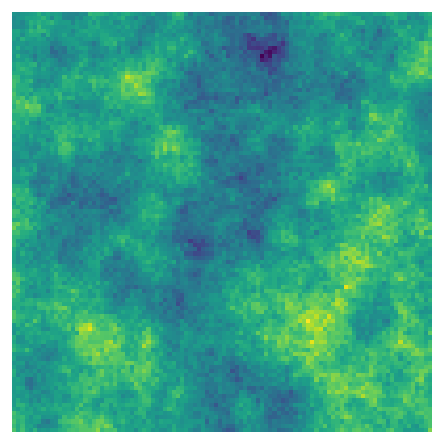
Each template gives a different kind of result. These six were run from the same menu (here by the command line, which runs the same files):


Open and run a template#
Let us open the simplest one. It finds the core of a forest, the part far enough from its edge that edge effects (more light, wind, predators, people) do not reach it, with GuidosToolbox's morphological spatial pattern analysis, MSPA (Soille & Vogt, 2009). You do not need to understand MSPA yet: the tutorial MSPA does that. Here it is only an example of a model.
- Click Templates, move to Patterns (GuidosToolbox) and click MSPA of a forest.
- Three nodes appear in the Model pane, joined from left to right, and run at once: the title bar says done in a few hundredths of a second.
- The Viewer shows the result, the template's Plot MSPA (the Viewer's header says Plot: MSPA): the forest split into core (green), edge (black), perforation (blue), islets, bridges, loops and branches.
- The node
mspais selected (orange outline), so the Node pane shows its settings.
The model is this graph. The same drawing appears in every tutorial of this site, with the model file under it (click Model file (TOML)):
Model file (TOML)
format = "terraflux/1"
name = "MSPA of a forest"

[[nodes]]
id = "landscape"
op = "nlm.random_cluster"
params = { rows = 300, columns = 300, p = 0.55, weights = [0.3, 0.15, 0.55], seed = 7 }
note = "A map of three classes drawn by chance (1 farming, 2 water, 3 forest): in its place, a raster.read of a map of yours."

[[nodes]]
id = "forest"
op = "raster.reclassify"
inputs = { map = "landscape.map" }
params = { rules = "3 -> 2\n* -> 1" }
note = "MSPA reads 2 as the foreground and 1 as the background: the forest (3) becomes 2, every other class 1."

[[nodes]]
id = "mspa"
op = "landscape.mspa"
inputs = { map = "forest.map" }
params = { edge_width = 1, connectivity = 8 }
note = "Core, islet, perforation, edge, loop, bridge and branch, as GuidosToolbox computes them."

[[plots]]
id = "plot"
title = "MSPA"
layers = [{ from = "mspa.map" }]
note = "Its map in the Viewer, in GuidosToolbox's colours, refreshed at every run."
Read it from left to right. Node 1, nlm.random_cluster, draws a landscape of 300 x 300 cells in three classes
(1 farming, 2 water, 3 forest). Node 2, raster.reclassify, turns the forest into 2 and everything else into 1,
because MSPA expects 2 for the habitat it analyses (the foreground) and 1 for the rest. Node 3,
landscape.mspa, runs MSPA. Each box lists its inputs on the left edge and its outputs on the right; the
connection from landscape.map to forest's input map is how the map travels. The [[plots]] at the end of the
model file is not a node: it is a Plot, a view of the result kept with the model, listed in the Viewer's
Plots menu (see Plots and figures).

Look at any step#
Click a node to select it: the Viewer shows what it gives. Click landscape and the Viewer shows the three classes
drawn by chance; click forest and you see the two classes MSPA reads. This is how you check a model step by
step: look at the output of every node before you trust the last one. A double click on a node shows its map in
the Viewer and keeps it as a layer, to keep it in view while you work on another node.
The small dot at the top right of a node tells how it did in the last run: green when it ran, a darker green when its result came from the cache (nothing it depends on had changed), orange while it runs, red when it failed.
Change a setting#
Select mspa. In the Node pane, under Settings, the box edge_width holds 1: the edge of the forest is one
cell wide. Click in it, type 3 and press Tab (or click elsewhere). Because update after every edit is
ticked, the model runs again at once: only mspa runs, landscape and forest come from the cache, and the
Viewer shows wider edges and smaller cores. Settings with a few possible values, such as
connectivity (8 or 4 neighbours), are chosen in a list instead.

Hover over the name of a setting to read what it means. Every setting of every operator is also in the operator reference.
Why a cell has its value: Trace#
Looking at every step tells you what each node gives. Trace answers a narrower question that comes up as soon
as a result surprises you: why does this cell have this value? Select mspa, click a cell of the forest's core
in the Viewer (the cell is outlined), and click Trace this cell in the bar above the map; a right click on the
cell offers the same in a menu. The Trace pane opens at the right of the window. At its top are the node and the
cell (its row, its column and its coordinates) and a sentence that sums up the answer; under it, a card per node,
from the cell back through the graph to the data, each with the node's value at that cell and how the node made it:
- for map algebra (
raster.calc), its expression, and the same expression with the cell's values in place of the names (2 if 1 == 1 and 0.71 > 0.45 else 1); - for an operator that reads the cells around (a moving window), the window of values around the cell;
- for an operator that works patch by patch (
raster.label,raster.sieve,landscape.mspa,metrics.patch...), the whole patch the cell is in: its class, how many cells it has, joined by 4 or 8 neighbours as the operator joins them, and the rows and columns it spans; its card's name draws the patch's border on the Viewer's map, around the cell (picking another cell lets it go). Here the card ofmspanames the patch offorest(class 2) the cell belongs to: a core cell is part of a patch of forest wide enough to have a core; - for an operator that uses the whole map (a regression fitted, a Markov chain), what it does, in a sentence;
- for the data read or drawn, nothing more: the chain ends there.
A card's name selects its node and shows that node's map in the Viewer with the same cell outlined, so you can
walk the chain on the maps themselves; the name of an input in a card jumps to that input's card. When the model
has a loop, Trace inside the loops runs it again keeping what the loop's nodes give at that cell, step by step.
A land change allocation (lulcc.step for CLUE-S and ordered allocation, dinamica.step for Dinamica EGO's
Expander and Patcher) then tells the steps at which the cell changed class and, at each, the step's demand (the
cells of each class, and how many more or fewer than at the step before) or the rate of its transition; a cell that
never changed says so. A line why tells what made the cell the one chosen: for CLUE-S, its suitability for each
class there, how the class it took ranks among the cells (above 92% of the cells) and the elasticity its own class
held it with (the iteration variable CLUE adds to each class until the demand is met is not kept by the step, and
the line says so); for Dinamica, its probability of that transition there and how it ranks, since the Expander
and the Patcher draw the cells of each change among the most probable. Inside a group, the node selected shows its map in the Viewer too, named by its place in the
group (preparation/temperature), and its cells are traced the same way.
Copy copies the trace as text. Ask the assistant why gives it to the application's assistant, to explain
in words; Explain with an MCP assistant, in the cell's right-click menu, keeps it for an assistant connected
through terraflux mcp and copies a request to paste in it (AI assistants).
The operators' library#
Terraflux has about 300 operators. There are three ways to add one to a model.
The drawer. Move the pointer to the left edge of the window: the Operators drawer slides out (the Files drawer has its own tab below it). At its top are your favourites, then the operators by subject, with a search box; files are opened with Ctrl+O (File > Open a raster or vectors...) or dragged from the Files drawer. Click an operator and a new node appears, already connected to the node selected, so a chain is built click after click.
The Operators menu in the toolbar holds the same library.
The search: /. Press / anywhere (when you are not typing in a box). A search opens over the
window; type part of an operator's name or of what it does (reclass, distance, core), choose with the
arrows, and press Enter: the operator is added after the node selected, and the new node becomes the selected
one. A chain of five nodes takes five searches, without the mouse. Esc closes the search.
The library is ordered by subject, the same subjects as the categories of this site's tutorials:
| Subject | Prefixes of its operators | For |
|---|---|---|
| IO | raster.read, raster.write, vector.read, vector.write |
reading and writing files |
| Data preparation | raster.*, vector.* |
reprojecting, resampling, clipping, reclassifying, rasterizing |
| Habitat patterns, Fragmentation | landscape.*, patterns.*, fragmentation.* |
GuidosToolbox |
| Landscape metrics | metrics.* |
landscapemetrics and FRAGSTATS |
| Habitat networks, Circuit connectivity, Grid distances | networks.*, conn.*, circuit.*, cost.* |
connectivity |
| Surface metrics, Distance & restoration, Change detection | surface.*, distance.*, restoration.*, change.* |
terrain, restoration, diffeR |
| Large data & batch | batch.* |
many files |
| Neutral landscape models | nlm.* |
NLMR's random maps |
| Biodiversity analysis, Spatial prioritization, Species distributions | bio.*, prioritize.*, sdm.* |
Biodiverse, Zonation, Marxan, linear programming, MaxNet |
| Land change simulation | markov.*, woe.*, dinamica.*, lulcc.*, plus.*, agents.*... |
Dinamica EGO, CLUE-S, PLUS, agents |
| Uncertainty | uncertainty.* |
Monte Carlo, error propagation |
| Map algebra, Model flow | map.*, stack.*, control.*, rng.*, plugin.* |
the pieces of every model (Building models) |
Favourites
Right-click an operator in the library to put it in a coloured collection of favourites (red, orange, yellow, green, blue, purple, grey). Your favourites are listed at the top of the drawer.
The data catalog#
File > Data catalog... (or "Data catalog" in Ctrl+K) lists the public datasets Terraflux downloads, a card
each: WorldClim 2.1 and CHELSA 2.1 (the climate of today and CMIP6 futures), the Copernicus DEM, SoilGrids 2.0,
MapBiomas Brazil, Hydrography90m, ESA WorldCover (land cover at 10 m), Hansen's Global Forest Change (tree cover,
the year of loss), MODIS (the vegetation indices NDVI and EVI every 16 days, the land surface temperature of the
day and of the night, the burned area by month, the yearly gross and net primary production) and GBIF's occurrences
of a species
(added as an sdm.download_gbif node). Search them (rain, soil, Brazil, future) or filter by theme. A card
says what the dataset holds, its resolution, years and coverage, its licence (WorldClim's is non-commercial,
CHELSA's public domain, Hydrography90m's non-commercial on its record) and the paper to cite, with a button that
copies it.
Choose what to fetch (the bioclimatic variables by name, the months, the scenario and period of a future, the
soil's property and depths, MapBiomas' years as 1985-2000, 2024) and the grid: a map of the model (by default
the first), the data then warped onto its extent, cells and coordinate system, or a box of longitudes and
latitudes. Cut to the area takes polygons the model gives (an area drawn on the map, a region read): no data
outside them, and the grid may then be the area's bounds (in longitudes and latitudes, widened to whole
cells). Add to the model adds a data.download node so set: it reads only the part the grid covers, once
(the files stay in the cache), and carries the dataset's reference, which Methods and citations lists. Under
the button, what is in the cache already for those choices (nothing to download, or so many layers); Preview
fetches the first layer over the grid, coarse (200 cells a side), and shows it before anything is added, or, for
GBIF, how many records it has.
The viewer#
Whatever the node selected gives is shown in the Viewer: a map with its legend, the layers of a stack one at a time (with < and > buttons and a slider), the maps of a loop's steps, a table (sortable, and drawn as bars, lines or points), or a single value. If the node has not run yet, the Viewer says so: Not run yet: ctrl+enter runs it, and what it needs.
Over a map:
- the wheel zooms around the pointer, dragging pans, a double click shows the whole map again;
- the corner shows the coordinates under the pointer, the row and column of the cell and its value (see Your first raster);
- Colours chooses a colour ramp (by default the colours fit the data: classes a colour each, values a ramp); cividis and orange to purple, centred on 0 read the same to colour-blind readers, and View > Colour vision draws every map and legend as a reader with protanopia, deuteranopia or tritanopia sees them, to check a figure before it is published (the bar at the top says so until you set it back);
- Compare puts another map beside this one: another output of the run (a scenario, another date, the observed map) or another layer of the same one (step 1 and step 50 of a simulation). As a Curtain, the other map is right of a line you drag across the map with its handle; Side by side, the two maps are in two views that zoom and pan together, a cross marking in one where the pointer is in the other. Both maps are drawn in the same colours (the classes of both, or one range from the lower minimum to the higher maximum), so that the same value is the same colour, and the corner reads out the values of both under the pointer. As a Difference, one map shows how they differ: for maps of values, the other map minus this one, in a ramp centred on 0 (with the mean difference and the share of cells higher and lower); for maps of classes, the transitions, a class each named by both legends ("forest -> pasture", the most common first, the cells that kept their class in grey), with how many cells changed. The difference is drawn where the map is, and Figure... can make a figure of it. A comparison worth keeping goes in the model: with it shown, choose Plots › Save as a new plot; the Plot opens with the comparison, and the report shows the two maps, and their difference when asked;
- Layers keep outputs on the map whatever node you click: the map shown is kept with the pin (a double click on a node keeps it too), Add a layer adds other maps and vector layers of the run, and each layer is shown or hidden, moved up or down, made more or less opaque (vectors styled) or taken away. A click on a layer's name shows that map, with its legend; the layers listed under it are drawn under it, those over it over it, and the pointer tells each map's value;
- Plots, in the Viewer's header, lists the model's Plots: a click opens one (its layers, the map shown, its comparison, a table's chart). Save as a new plot keeps what the Viewer shows with the model; with a Plot open, the menu also holds its title, Update the plot and Remove the plot. The Document and the report show the Plots as figures (see Plots and figures);
- clicking a cell lists, under This cell in every map, its value in every map of the run at the same place (placed by their coordinates; outside where a map does not reach it): the land cover, the elevation and the model's result of one place side by side. A name shows that map, and Copy copies the list;
- clicking a cell of a stack draws a chart of that cell's value in every layer.
Figure..., at the top of the panel beside the map, makes a figure for a paper of the map shown: alone, beside the map compared, or every layer of a stack or a series as panels (a), (b)... in columns. Give it a title, the width (85 mm is a journal's column, 180 mm its page) and the resolution (300 or 600 DPI, as journals ask), and choose the legend, the scale bar (in metres or kilometres, also on a map in longitudes and latitudes), the north arrow, the coordinates along the edges and the location inset (a small map of the world around, the map's place in red, in its bottom right corner); the preview follows. The vector layers drawn over the map (in Layers) are drawn over it in the figure too, in their colours, cut at the map's edge. Save PNG... records the resolution in the file, so that a word processor places it at its width; Save SVG... keeps the text as text, to change in Inkscape or Illustrator; Save PDF... writes a PDF of the figure's size, its lines and text as lines and text (in Helvetica) and the maps as pictures.
A map of several layers (a stack, the steps of a loop, the bands of a raster) has Play beside its slider (the layers one after another, again and again; the arrows or the slider stop it), a speed in frames a second (the same for playing and for saving, and for the Simulation pane), and Save as GIF... under them: the layers as an animated GIF, for a talk or a class, each with its name in its corner and its legend under it. Save as MP4... saves the same frames as a video (H.264, made by terraflux itself: nothing to install), which slides and video players take. The steps of a series share one set of colours, so that a value keeps its colour from step to step; the layers of a stack or a raster (often different variables) each keep their own, as the Viewer shows them. The Simulation pane has the same buttons for the steps of a run (step 12 of 50) and for the maps of an input's stack. A small map is enlarged, a large one is read every few cells (at most 800 pixels a side), and the animation is made in the background while you keep working.
Basemaps#
Under Basemap you can put a map of the world under your data: Satellite (Esri), Topographic (Esri), OpenStreetMap, OpenTopoMap or Light (Carto). Terraflux downloads the tiles, reprojects them onto your map's coordinate system and keeps them in a cache on your computer. show the data and its opacity slider let you see through your map to the imagery: the quickest way to check that a land cover map is where it should be, and whether its forest really is forest. With the pointer over a map, the key B puts the satellite imagery under it (and B again takes it away).
A basemap needs coordinates
A basemap can only be placed under a map that has a coordinate reference system (CRS): it must know where on Earth the cells are. The templates' maps are drawn by chance, on no place, so they have none; a GeoTIFF of a real place usually has one. A basemap also needs an Internet connection the first time an area is shown. See Coordinate systems for files without a CRS.
The model as a document#
Beside the Model pane's tab is the Document tab: the same model read as the methods section of a paper, for
whoever reads, checks or reviews it rather than builds it. Its nodes are told in stages (Data, Preparation,
Model, Validation, Results), a step each, with its note, a sentence of what it does with its settings and
where its inputs come from ("MSPA's patterns of forest: connected by 8 neighbours, the edges 1 cell wide."), its
settings, and its map or table from the last run; the model's Plots are its numbered figures. A step's name selects its
node, and a setting can be changed there as in the Node pane. Export report writes it as a web page or a PDF (in English or Portuguese),
and Methods and citations drafts the methods section of a paper from the model, with the papers to cite, in
English or Portuguese (also terraflux methods model.toml --language pt on the
command line, and the methods tool of the AI assistants).
File > Export to QGIS... writes the run's maps, in their colours, as a QGIS project
(Opening the results in QGIS).
The model's document explains it all.
File > Python script (landschaft)... writes the model as a Python script of
landschaft, the library whose methods Terraflux runs, for the paper's
code availability, a supervisor or a reviewer who asks for the code: a call of landschaft a node, in the order the
model runs them, its note as a comment and its settings as the function's arguments. A calculator keeps its script,
run in numpy by a helper written at the top of the file; reclassification rules become ls.reclassify's table, and
the foreground of MSPA, FAD and the other patterns ls.reclassify(map, foreground=...). Containers become
Python's own: a loop a for over its steps (what it carries assigned at the end of each step, what it collects
appended to a list, its end a break), a loop over a collection a for over its elements, a switch an if per
branch, a group its body in place. A species distribution model becomes landschaft's prepare, fit and
predict; landscape metrics ls.landscape_metrics; a prioritization prioritizr's problem() chain as landschaft
builds it (objective, targets, penalties, constraints, the solver), Zonation ls.prioritize.zonation; Markov
chains and weights of evidence their landschaft classes. The window says how many nodes were translated; a node
without a counterpart known yet stays as a comment with its settings, to write by hand (the allocation of
Dinamica, CLUE-S and PLUS, which landschaft runs only as a whole model with ls.simulate.run, says so). The
neutral landscapes, the calculator, the reclassification, GuidosToolbox's patterns, Zonation, the prioritization,
the species distribution model and the loops give the same maps as the model (the same seeds: NLMR's maps).
The Changes pane#
The Changes pane (View > Changes) lists what changed in the model since an earlier version of it, node by node, each change to keep or undo: what an AI assistant changed, or the differences with the saved file, with a commit of the model's file in git, or with another model file (File > Compare). For a node changed, it shows its map or table before and now, side by side. AI assistants explains it.
Settings#
⚙ at the right of the toolbar opens the settings, a small window:
- Theme: the colours of the window. The classic themes (Default, Immaterial, Field Notes, Riparian, Angst Robot, Twenty Four Carat) keep the square look; the modern ones (Slate, dark; Paper, light, in the colours of this website; Canopy, dark green) have rounded panes and cards, switches and a font of their own;
- Text size and Interface zoom: for a small laptop screen or a projector;
- Threads: how many of the computer's cores the operators use. By default all the cores but one, so that the computer stays usable while a model runs; the change takes effect at the next start.
Settings, favourites and the layout are kept in your user's application data (%APPDATA%\Terraflux on Windows,
~/Library/Application Support/Terraflux on macOS, ~/.config/Terraflux on Linux).
The keys worth learning#
| Key | Does |
|---|---|
| F5 | run the whole model |
| Ctrl+Enter | run up to the node selected (what it needs, the rest from the cache) |
| / | search the operators and add one after the node selected |
| Ctrl+O | open a raster or vectors |
| Ctrl+S | save the model |
| Ctrl+L | arrange the nodes in tidy columns |
| Ctrl+R | rename the node selected |
| Del or Backspace | delete the nodes selected |
| Tab | go to the Model pane, and Tab again back to where you were |
| Ctrl+W | close the tab in front |
| Home | fit the whole graph in the canvas |
| B (over a map) | satellite imagery under the map, or none |
| arrows (over the canvas) | go to the node beside the one selected; Enter shows its output |
On macOS, Cmd takes the place of Ctrl.
Common pitfalls#
- Nothing happens when I press a key. Keys go to the pane under the pointer, and not while you type in a box: click on the canvas first.
- The map I expect is not shown. The Viewer shows the node selected. Click the node whose output you want, or double-click it to bring the Viewer to the front with it.
- A required input is missing. Inputs that must be connected are marked with a star in the Node pane and are drawn in orange on the canvas until they are; Run stays greyed out while a model has errors, which the Model pane's Text view lists.
- A template's result looks random. It is: the templates draw their maps by chance (with a fixed seed, so
the same map each time). Replace the first node by a
raster.readof your own map to use real data; the Quickstart does it. - A pane disappeared. Turn it back on in View, or View > Reset the layout.
Going further#
- Your first raster: what the numbers in the viewer mean.
- Your first model: build a model by hand, connect its nodes, save it and run it from the command line.
- Building models: map algebra, stacks, loops, groups and plugins.
- The Glossary and the operator reference.
References#
- Gardner, R. H., Milne, B. T., Turner, M. G., & O'Neill, R. V. (1987). Neutral models for the analysis of broad-scale landscape pattern. Landscape Ecology, 1(1), 19–28. https://doi.org/10.1007/BF02275262
- Sciaini, M., Fritsch, M., Scherer, C., & Simpkins, C. E. (2018). NLMR and landscapetools: An integrated environment for simulating and modifying neutral landscape models in R. Methods in Ecology and Evolution, 9(11), 2240–2248. https://doi.org/10.1111/2041-210X.13076
- Soares-Filho, B. S., Coutinho Cerqueira, G., & Lopes Pennachin, C. (2002). DINAMICA: a stochastic cellular automata model designed to simulate the landscape dynamics in an Amazonian colonization frontier. Ecological Modelling, 154(3), 217–235. https://doi.org/10.1016/S0304-3800(02)00059-5
- Soille, P., & Vogt, P. (2009). Morphological segmentation of binary patterns. Pattern Recognition Letters, 30(4), 456–459. https://doi.org/10.1016/j.patrec.2008.10.015