Connectivity, contagion and mosaics at a fixed scale

Part 1 measured how much forest surrounds every forest cell. Two forest cells with 60% forest around them can be in very different places: at the straight edge of a large block, or in a scatter of small woods. This part measures the arrangement of the forest in the window as well as its amount, with GuidosToolbox's fragmentation at a fixed observation scale (FOS), Riitters' classic model of density and contagion, and the spatial entropy; then extends the window to maps of % tree cover (GraySpatCon) and to the landscape mosaic, which asks what the rest of the window is: fields or towns. At the end you will be able to choose among GuidosToolbox's indices for a question, map them, and read their reports.

The idea#

Density, edges and clustering#

FOS computes, for every forest cell, a connectivity of the forest in the window around it, from 0 to 100%, in one of three ways (Vogt & Riitters, 2017):

Method	What it counts in the window	High when
FAD, forest area density	the share of forest (part 1)	there is much forest
FED, forest edge density	the edges between forest and the rest (GraySpatCon's clustering of the forest)	the forest has little edge for its amount
FAC, forest area clustering	the pairs of neighbouring cells that are both forest, among all pairs with data	the forest is in compact blocks

All three are reported in GuidosToolbox's classes, the same as FAD's: rare, patchy, transitional, dominant, interior and intact (or five classes, intact merged into interior). GuidosToolbox's report calls fragmentation the complement, \(100\% - \text{connectivity}\).

Key idea: density and contagion

Riitters et al. (2000) described the forest in the window around every forest cell by two probabilities:

\(P_f\), the share of the window that is forest: FAD (here divided by 100);
\(P_{ff}\), the contagion: of the pairs of neighbouring cells in the window that include a forest cell, the share in which both are forest. If you stand on forest in that window, the chance your neighbour is forest too.

Together they place every cell in one of six categories: interior (\(P_f = 1\)), patch (\(P_f < 0.4\)), transitional (\(0.4 \le P_f < 0.6\)), and for \(P_f \ge 0.6\), edge when \(P_f > P_{ff}\) (the forest's non-forest neighbours are on one side, as at the edge of a block), perforated when \(P_f < P_{ff}\) (the gaps are holes inside the forest), and undetermined when they are equal. The model was used for the first global map of forest fragmentation (Riitters et al., 2000) and for the forests of the United States (Riitters et al., 2002).

Entropy#

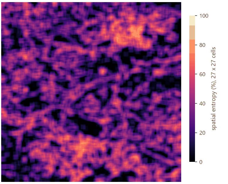
Spatial joint entropy measures how mixed neighbouring cells are, from the pairs of neighbours: 0% when the map is one class, 100% when forest and non-forest neighbours are as mixed as they can be. For the whole map it is one number; in a moving window, a map of where the forest and the rest are most intermingled.

% cover maps#

Not every habitat is a yes-or-no. Maps of % tree cover (or % impervious surface, % cropland) are continuous, and binarizing them at a threshold throws information away. GuidosToolbox's FOS reads such maps directly (values 0 to 100, 255 missing): the foreground is the cover from a threshold up, and the connectivity the mean cover in the window (FAD) or its clustering (FED). GraySpatCon (Riitters and Vogt's moving-window program for % maps, part of GuidosToolbox) computes more: the mean, median, standard deviation, Shannon's diversity or evenness of the cover around every cell.

The landscape mosaic#

Density says how much forest surrounds a cell, not what the rest is. Is the forest surrounded by farmland or by suburbs? The landscape mosaic (Riitters et al., 2009) describes every window by its shares of three land covers, agriculture, natural and developed, and places it in a triangle of compositions divided into 19 classes: pure (100% of one), dominated (more than 60% of one, named by the others present), and mosaics (none above 60%). The mosaic captures the human context of the habitat, which decides the kind of edge effects it receives: a crop field and a road do not make the same edge.

When to use it#

FOS-FAC or FED to tell a forest cell inside a compact block from one in a scatter of small woods at the same density; to report the connectivity of a forest at one scale, with GuidosToolbox's report (ECA, coherence).
Riitters' model to map edge versus perforation: whether a forest is being eaten from its edges or pierced from within.
Entropy to compare how intermingled maps or regions are.
% cover maps (FOS on gray maps, GraySpatCon) for tree cover products such as Global Forest Watch's, without choosing one threshold.
The landscape mosaic for the human context of habitat: the threat a forest's neighbourhood poses (Riitters et al., 2012), the urbanization of a region.
Not for the structural role of cells (MSPA) or connectivity for a species (habitat networks).

What you need#

As in part 1, a map coded 0 missing, 1 background, 2 forest, or classes given in foreground: input.tif. For % cover, a map of 0–100 with 255 missing: GraySpatCon's sample, a map of tree cover of the conterminous United States at 2.43 km (1,289 × 1,990 cells), shipped with landschaft. For the mosaic, a land cover: clc.tif, CORINE around Hannover. In the application, Templates > Patterns (GuidosToolbox) > Fragmentation of a forest has FOS by FAC; Landscape mosaic has the mosaic, contagion and entropy.

FOS: density, edges and clustering#

Build the model#

The forest's connectivity in windows of 27 cells by FAD, FED and FAC.

Model file (TOML)

format = "terraflux/1"

[[nodes]]
id = "forest"
op = "raster.read"
params = { path = "input.tif" }

[[nodes]]
id = "fos_fad"
op = "fragmentation.fos"
inputs = { map = "forest.raster" }
params = { window = 27, method = "FAD", classes = 6 }

[[nodes]]
id = "fos_fed"
op = "fragmentation.fos"
inputs = { map = "forest.raster" }
params = { window = 27, method = "FED", classes = 6 }

[[nodes]]
id = "fos_fac"
op = "fragmentation.fos"
inputs = { map = "forest.raster" }
params = { window = 27, method = "FAC", classes = 6 }
note = "Clustering: forest-forest pairs."

fragmentation.fos takes the map and four settings that matter: window (the side in cells, odd), method (FAD, FED or FAC), classes (5 or 6: whether intact is apart from interior) and connectivity (8 or 4, for counting the patches of the report). Its outputs: map (the connectivity, 0–100%, on the forest; 101 background, 102 missing), stats (the share of the forest in each class), summary and report (GuidosToolbox's report, below).

Read the results#

Method	Intact	Interior	Dominant	Transitional	Patchy	Rare	Average
FAD	7.3	32.7	32.2	14.0	12.2	1.6	73.5%
FED	12.5	28.4	32.0	13.7	12.1	1.5	73.9%
FAC	6.9	30.1	31.4	14.6	13.8	3.2	70.6%

FOS by FAD gives exactly the numbers of FAD in part 1: the same index. FED classes more of the forest as intact (12.5%) and less as interior: it measures the forest's edges in the window rather than its area. FAC is the strictest: thin strips of forest, whose cells have many non-forest neighbours, fall to patchy and rare (3.2% rare against 1.6%). With five classes, intact and interior merge (37.0% for FAC).

GuidosToolbox's report#

The report output is GuidosToolbox's text report, the same file it writes (fos.txt); select the node to see it, or make it an output of the model. For FAC at 27 cells:

FOS parameter settings:
Binary
Foreground connectivity: 8-connectivity
FOS-type selected: FAC_6class
Pixel resolution [m]: 25
Window size [pixels]: 27
Observation scale [(window size * pixel resolution)^2]: 45.5625 hectares <-> 112.587 acres
...
A) Image summary:
Reporting unit area [pixels]: 999730
Foreground area [pixels]: 428490
Foreground area [%]: 42.8606
Number of foreground patches: 2850
Average foreground patch size [pixels]: 150.347
B) Reporting levels
- Average FAC at WS27 [%]: 70.5904
- ECA (Equivalent Connected Area) [pixels]: 221293
- COH (Coherence = ECA/ECA_max*100) [%]: 51.6448
- AVCON (average connectivity) at WS27 [%]: 30.2554
- COH_ru (ECA/Reporting unit area*100) [%]: 22.1353

(The full report: fos-report.txt.) Its reporting levels are the numbers to put in a table:

Average FAC: the mean connectivity of the forest's cells, 70.6%.
ECA: the equivalent connected area of the forest's patches, \(\sqrt{\sum a_i^2}\), the size of one patch that would offer as much reachable forest (see habitat patterns, part 4); COH, ECA over the total forest: 51.6%, so the forest behaves as half of one block.
AVCON: the average connectivity over the whole reporting area, forest or not: 30.3%. It falls with both the loss of forest and its fragmentation.
COH_ru: ECA over the reporting area.

pixel_resolution sets the cell size used in the report's hectares (default 25 m): set it to your map's.

How the window changes the answer#

Window (cells) 5 — FOS by FAC in the south of the map at windows from 5 to 135 cells. At small windows most of the forest is intact; as the window grows, the large forests turn interior then dominant, and the valley's woods transitional and patchy. Numbers: % of the whole forest in each class, and the average connectivity.

Window (cells) 9 — FOS by FAC in the south of the map at windows from 5 to 135 cells. At small windows most of the forest is intact; as the window grows, the large forests turn interior then dominant, and the valley's woods transitional and patchy. Numbers: % of the whole forest in each class, and the average connectivity.

The stacked chart is the forest's fragmentation profile: the intact share vanishes by 45 cells, the interior share peaks at about 27 cells and then shrinks, and transitional and patchy grow steadily. Two forests can have the same profile at one window and different ones at another; a profile over several windows is the most complete description.

Choosing the window. GuidosToolbox's FAD-MS uses 7, 13, 27, 81 and 243 cells; with 25 m cells, from 3 ha to 3,700 ha. For one scale, choose it from the process: the depth of edge effects on microclimate (tens of metres), the home range of a forest bird (a few hectares to tens), the area of a mammal's territory (hundreds of hectares). And report it in metres and hectares, not only in cells: the report does the conversion with pixel_resolution.

Density and contagion: Riitters' model#

The forest's density and contagion in windows of 7 cells, the two axes of Riitters et al.'s model; and the spatial entropy, of the whole map and in windows of 27 cells.

Model file (TOML)

format = "terraflux/1"

[[nodes]]
id = "forest"
op = "raster.read"
params = { path = "input.tif" }

[[nodes]]
id = "density"
op = "fragmentation.fad"
inputs = { map = "forest.raster" }
params = { window = 7 }
note = "Pf x 100."

[[nodes]]
id = "contagion"
op = "fragmentation.contagion"
inputs = { map = "forest.raster" }
params = { window = 7 }
note = "Pff x 100."

[[nodes]]
id = "entropy"
op = "fragmentation.entropy"
inputs = { map = "forest.raster" }
note = "One number for the map."

[[nodes]]
id = "entropy_map"
op = "fragmentation.entropy_map"
inputs = { map = "forest.raster" }
params = { window = 27 }

Riitters' categories are a rule on two maps of the same window: node 2's density and node 3's contagion. With raster.calc the rule is one expression; here we drew it from the two maps:

Density against contagion — Every forest cell of the map by its density (Pf) and contagion (Pff) in a window of 7 cells (a log scale of counts). The diagonal separates edge (below: the window's non-forest is on one side) from perforated (above: holes inside the forest); the dashed lines separate patch, transitional and the rest.

Over the whole map: interior 51.7% of the forest, perforated 18.3%, edge 11.5%, transitional 8.4%, patch 7.1%, undetermined 3.1%. A forest whose loss comes as perforation (clearings inside it) and one whose loss comes from its edges inwards have the same FAD and different categories; the change between dates shows which is happening.

fragmentation.contagion and fragmentation.clustering (FAC as a plain map) take the map and window; both give the % on the forest and GuidosToolbox's codes elsewhere.

Entropy#

fragmentation.entropy gives one number, the spatial joint entropy of the whole map: 32.5% here, a map far from maximally mixed; its pairs table counts every kind of pair of neighbours. fragmentation.entropy_map computes it in a window around every cell:

% cover: tree cover of the United States#

FOS of a % tree cover map, and GraySpatCon's standard deviation of the cover around every cell.

Model file (TOML)

format = "terraflux/1"

[[nodes]]
id = "cover"
op = "raster.read"
params = { path = "gscinput.tif" }
note = "% tree cover, 255 missing."

[[nodes]]
id = "fos"
op = "fragmentation.fos"
inputs = { map = "cover.raster" }
params = { window = 7, method = "FAD", gray_threshold = 30 }
note = "Forest: 30% cover or more."

[[nodes]]
id = "variability"
op = "fragmentation.gray_convolution"
inputs = { map = "cover.raster" }
params = { metric = "stddev", window = 7 }

fragmentation.fos recognises a % cover map by its values (above 4); grayscale = true forces it. The gray_threshold (default 30) decides which cells are forest, but the connectivity uses the cover itself: with FAD, it is the mean cover in the window. fragmentation.gray_convolution computes one of GraySpatCon's metrics of the cover in the window (mean, median, majority, min, max, range, stddev, shannon_diversity, shannon_evenness, diagonal_contagion).

Forest (30% cover or more) is 29.0% of the area with data, in 17,785 patches. Its average connectivity (the mean cover around forest cells) is 49.7%: dominant 38.3% of the forest, transitional 29.8%, patchy 28.8%, rare 2.9%, and interior a mere 0.2% (a window of 17 km with 90% mean cover is rare at this resolution).

The landscape mosaic#

CORINE's classes grouped into agriculture, natural and developed land, and the landscape mosaic in windows of 27 cells (675 m).

Model file (TOML)

format = "terraflux/1"

[[nodes]]
id = "corine"
op = "raster.read"
params = { path = "clc.tif" }

[[nodes]]
id = "mosaic"
op = "fragmentation.landscape_mosaic"
inputs = { map = "corine.raster" }
params = { window = 27, agriculture = [12, 13, 14, 15, 16, 17, 18, 19, 20, 21, 22], natural = [23, 24, 25, 26, 27, 28, 29, 30, 31, 32, 33, 34, 35, 36, 37, 38, 39], developed = [1, 2, 3, 4, 5, 6, 7, 8, 9, 10, 11] }
note = "Water (40-44) is in none: missing."

fragmentation.landscape_mosaic takes a land cover and the classes of each of the three groups (or a map already coded 1 agriculture, 2 natural, 3 developed). Classes in no group are missing: here water, which is neither a pressure nor a habitat for this question. Its outputs: map (19 classes, or 103 with classes = 103), stats (the cells of each of the 103 classes and its class of 19), heatmap and triangle (the shares on GuidosToolbox's triangle), heatmap_csv (GuidosToolbox's heatmap.csv).

The mosaic's heatmap — GuidosToolbox's heatmap: every window as a point in the triangle of compositions (natural at the top, developed bottom left, agriculture bottom right), the colour the share of the cells in each part of the triangle (a log scale). The landscape is concentrated in the pure corners and along the edges of the triangle (mixes of two groups); mixes of all three are rare.

The largest classes: pure agriculture 28.7% of the cells with data, agriculture above 60% with some of the others 12.3%, agriculture–developed 9.4%, agriculture–natural 8.8%, pure natural 8.6%, pure developed 5.0%. Riitters et al. (2009) followed the shift of the United States' forests through this triangle between dates: forests moving towards the developed corner are under pressures that their density alone does not show.

Reading the class names

A name lists the classes from the most abundant: Forest-Agriculture is a natural cover above 60% with agriculture as the second class (10% or more), Forest-Agriculture-Developed the same with developed land at 10% or more too, and Mosaic ... a mix where no class reaches 60%. Report the class numbers with their names.

Settings that change the answer#

The window, above; and the cell size it multiplies.
The method of FOS: FAD measures amount, FED edge, FAC clustering. Say which.
5 or 6 classes: intact apart or not.
The threshold of a % cover map (gray_threshold): which cells are forest.
The groups of the mosaic: what counts as natural (are pastures agriculture or natural?) changes every class.
Missing data: left out of the windows' counts. Large areas of missing data (water, outside a country) shrink the windows near them.

Common pitfalls#

Comparing FOS of different methods or windows. The classes have the same names, not the same meaning.
A % map read as binary. A map of 0–100 is read as % cover automatically; a binary map coded 0/½ that also has larger codes may be taken for % cover: check the report's first line (Binary or Grayscale).
The report's hectares. They use pixel_resolution (25 m by default), not the map's cell size.
Entropy across maps of different amounts. Entropy is highest at 50% forest; compare it between maps with similar amounts, or read it with FAD.
A mosaic with water as natural. Water counted as natural makes lakes "natural cores". Leave it out unless it is part of the question.

Going further#

Part 3: how these indices change between two dates.
Landscape metrics, moving windows: any landscape metric in a window.
Habitat patterns: MSPA's classes of the same forest.
The operator reference: fragmentation.fos, fragmentation.contagion, fragmentation.clustering, fragmentation.entropy, fragmentation.entropy_map, fragmentation.gray_convolution, fragmentation.landscape_mosaic.

References#

Riitters, K., Wickham, J., O'Neill, R., Jones, B., & Smith, E. (2000). Global-scale patterns of forest fragmentation. Conservation Ecology, 4(2), 3. https://doi.org/10.5751/ES-00209-040203
Riitters, K. H., O'Neill, R. V., Wickham, J. D., & Jones, K. B. (1996). A note on contagion indices for landscape analysis. Landscape Ecology, 11(4), 197–202. https://doi.org/10.1007/BF02071810
Riitters, K. H., Wickham, J. D., O'Neill, R. V., Jones, K. B., Smith, E. R., Coulston, J. W., et al. (2002). Fragmentation of continental United States forests. Ecosystems, 5(8), 815–822. https://doi.org/10.1007/s10021-002-0209-2
Riitters, K. H., Wickham, J. D., & Wade, T. G. (2009). An indicator of forest dynamics using a shifting landscape mosaic. Ecological Indicators, 9(1), 107–117. https://doi.org/10.1016/j.ecolind.2008.02.003
Riitters, K. H., Wickham, J. D., Wade, T. G., & Vogt, P. (2012). Global survey of anthropogenic neighborhood threats to conservation of grass-shrub and forest vegetation. Journal of Environmental Management, 97, 116–121. https://doi.org/10.1016/j.jenvman.2011.11.009
Vogt, P., & Riitters, K. (2017). GuidosToolbox: universal digital image object analysis. European Journal of Remote Sensing, 50(1), 352–361. https://doi.org/10.1080/22797254.2017.1330650
Vogt, P., Riitters, K., Rambaud, P., d'Annunzio, R., Lindquist, E., & Pekkarinen, A. (2022). GuidosToolbox Workbench: spatial analysis of raster maps for ecological applications. Ecography, 2022(3), e05864. https://doi.org/10.1111/ecog.05864