Neutral landscape models

A neutral landscape is a map drawn by chance, with known rules and nothing else: no rivers, no roads, no history. That sounds useless to an ecologist, and it is the opposite. Because we know exactly how a neutral landscape was made, it tells us what pattern chance alone would give, and so what in a real landscape needs another explanation. It lets us make many landscapes that differ in one property only, the amount of habitat or its fragmentation, to see how a species or a metric responds. And it gives every tool something to run on before the real data arrive. This first part explains the idea and its history, shows every generator of Terraflux side by side, and moves the settings that control the pattern; part 2 uses them in a study. At the end you will know which model to choose for which purpose and how to set it.

The idea#

A null model for landscapes#

Ecology uses null models to ask whether a pattern is more than chance: are these species found together more often than random draws would give? Gardner et al. (1987) brought the idea to landscapes. They drew maps in which every cell is habitat with a probability \(p\), independently of the others, and measured the clusters of habitat: how many, how large, whether one crossed the map. Real landscapes could then be compared with these neutral expectations: a real forest more aggregated than a random map of the same amount is aggregated for a reason (soils, topography, history), and that reason becomes the question.

The random map was soon joined by maps with structure. Fractal landscapes, rough or smooth, spatially autocorrelated as real ones are, were used to study how species respond to the amount and the fragmentation of habitat (With & Crist, 1995; With, 1997). The modified random clusters of Saura and Martínez-Millán (2000) gave patches with irregular, realistic shapes and controlled amounts of several classes. Software then gathered the models in libraries: NLMpy in Python (Etherington et al., 2015) and NLMR in R (Sciaini et al., 2018). Terraflux implements NLMR's models with its settings, and for the same seed draws the same map as NLMR does.

Key idea: percolation

On a random map, the habitat's clusters grow with \(p\), the share of habitat, but not gradually. Below a critical share \(p_c\) the clusters are small and separate; just above it, one cluster suddenly spans the map (Gardner et al., 1987; Stauffer & Aharony, 1994). For an infinite square grid, \(p_c \approx 0.593\) when cells connect by their sides (4 neighbours) and \(p_c \approx 0.407\) when corners count too (8 neighbours). The threshold is a property of random maps; on autocorrelated maps habitat connects at lower amounts. Its lesson for real landscapes: connectivity can collapse after a small loss of habitat, near a threshold.

What makes a model neutral#

A neutral landscape model has three ingredients:

a surface or a process drawn by chance: independent values, values correlated over a distance, a fractal, a gradient, a tessellation of polygons;
settings that control its pattern: the share of habitat, the size of clusters, the roughness;
a seed for the random numbers: the same seed and settings give the same map, another seed gives another map with the same properties, a replicate.

Many models draw a continuous surface from 0 to 1. A binarization cuts it at a share of habitat (the highest cells become habitat), and a classification cuts it into classes of given shares. The amount is then exactly controlled, and the surface controls only the arrangement.

When to use it#

As a null model: is the aggregation, the shape or the connectivity of a real habitat more than chance? (part 2)
As an experiment: landscapes that vary in amount and fragmentation independently, with replicates, to see how a metric, a dispersal model or a population model responds; impossible with real landscapes, where the two go together (Fahrig, 2003).
As test data: every model of this site that starts from a template draws its landscape with these models, so that it runs at once; replace them by your maps later.
Not as a prediction of a real landscape: a neutral landscape has the statistical properties you set, not the history of a place.

What you need#

Nothing but Terraflux: these models make their own maps. Each takes the size (rows, columns), the cell's side (resolution, so that metrics come out in hectares and metres) and a seed; or, connected to the input like, the grid of another map, to draw a neutral landscape on the grid of a real one. In the application, the library's subject Neutral landscape models has them all; the templates Templates > Surfaces and uncertainty > Neutral landscapes (three of them) and More neutral landscapes (the others and the utilities) show them side by side.

Every generator#

Three neutral landscapes side by side: a random cluster of three classes, a Gaussian field and a fractal surface (the template Neutral landscapes).

Model file (TOML)

format = "terraflux/1"

[[nodes]]
id = "clusters"
op = "nlm.random_cluster"
params = { rows = 256, columns = 256, p = 0.4, weights = [0.25, 0.25, 0.5], seed = 4 }
note = "Classes: a colour each."

[[nodes]]
id = "field"
op = "nlm.gaussian_field"
params = { rows = 256, columns = 256, range = 20, seed = 4 }
note = "Values from 0 to 1."

[[nodes]]
id = "fractal"
op = "nlm.fbm"
params = { rows = 256, columns = 256, dimension = 1.5, seed = 4 }

[[plots]]
id = "plot_clusters"
layers = [{ from = "clusters.map" }]

[[plots]]
id = "plot_field"
layers = [{ from = "field.map" }]

[[plots]]
id = "plot_fractal"
layers = [{ from = "fractal.map" }]

Each generator is one node without inputs: add it from the library, set its size and seed in the Node pane, and click it to see its map in the Viewer. The template keeps each map as a Plot (the Viewer's Plots menu). Here are all fifteen, on grids of 200 × 200 cells.

What each draws, and what it is good for:

Generator	Draws	Good for
`nlm.random`	an independent value in every cell	the null model without any structure
`nlm.percolation`	habitat (1) with probability `prob`, else 0	Gardner's random maps, percolation
`nlm.planar_gradient`	a linear gradient along `direction`	a climate, an altitude, a distance from a coast
`nlm.edge_gradient`	a gradient peaking in the middle of the map	a ridge, a valley floor
`nlm.distance_gradient`	the distance to a rectangle (`origin`)	the distance from a town or a source
`nlm.mpd`	a fractal by midpoint displacement (`roughness` 0 smooth to 1 rough)	classic fractal landscapes (Palmer, 1992)
`nlm.fbm`	fractional Brownian motion (`dimension`, small rough, large smooth)	fractal landscapes of controlled roughness (Keitt, 2000)
`nlm.gaussian_field`	a smooth surface autocorrelated over `range` cells	environmental surfaces, suitability, drivers
`nlm.random_cluster`	patches of classes with irregular shapes (`p`, `weights`)	realistic maps of land cover classes
`nlm.neigh`	categories grown from their neighbours	patchy maps of several categories
`nlm.random_rectangular_cluster`	overlapping rectangles	fields, plots, human land use
`nlm.curds`	hierarchical blocks of habitat (`curds`, `steps`)	habitat structured at several scales
`nlm.mosaic_tess`	Voronoi polygons of random values	polygon mosaics, parcels
`nlm.mosaic_gibbs`	Voronoi polygons from germs kept apart, in classes	mosaics of regular polygons
`nlm.mosaic_field`	the sum of random line tessellations	linear structures, faults

And four utilities turn surfaces into maps: nlm.binarize (habitat and matrix at a share), nlm.classify (classes of given shares, of a real map's shares, or by natural breaks), nlm.merge (a surface plus others times a scaling: a gradient with noise) and nlm.rescale (to 0–1).

Percolation: when habitat connects#

A random map of 57.5% habitat and its patches by 4 neighbours, with the area of each.

Model file (TOML)

format = "terraflux/1"

[[nodes]]
id = "random"
op = "nlm.percolation"
params = { rows = 200, columns = 200, prob = 0.575, seed = 1 }
note = "Habitat (1) with probability 0.575."

[[nodes]]
id = "patches"
op = "metrics.patch"
inputs = { map = "random.map" }
params = { metrics = ["area"], directions = 4, show = "area" }
note = "The largest cluster is the patch of largest area."

nlm.percolation's prob is the share of habitat. metrics.patch (landscape metrics) labels its clusters; directions = 4 connects cells by their sides only. Move the slider through the threshold:

Habitat (share of the cells) 0.45 — Random maps of 200 × 200 cells with growing shares of habitat (light green), their largest cluster by 4 neighbours in dark green. At 55% the largest cluster holds 4% of the habitat; at 57.5% it suddenly spans the map; at 62.5% it holds most of the habitat.

Habitat (share of the cells) 0.5 — Random maps of 200 × 200 cells with growing shares of habitat (light green), their largest cluster by 4 neighbours in dark green. At 55% the largest cluster holds 4% of the habitat; at 57.5% it suddenly spans the map; at 62.5% it holds most of the habitat.

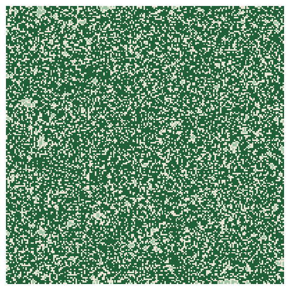
Over ten replicates (seeds 1 to 10) and both neighbour rules, the curve is the same:

The share of the habitat in its largest cluster, the mean of 10 random maps of 200 × 200 cells at each amount. With 8 neighbours the habitat connects between 37.5 and 42.5% (the threshold 40.7%); with 4, between 57.5 and 62.5% (59.3%). A few percent of habitat more or less, near the threshold, decide whether the landscape is one network or dust.

With & Crist (1995) and With (1997) showed that species respond to such thresholds, at amounts that depend on how they move: a species that crosses gaps of one cell sees the 8-neighbour curve, or an even lower one. And real habitat, being aggregated, connects at lower amounts than random habitat: the next sections draw such landscapes.

Settings that change the pattern#

The random cluster's p#

nlm.random_cluster (Saura & Martínez-Millán, 2000) first makes a random map with a share p of cells, joins them into clusters, gives each cluster a class drawn with the weights, and fills the remaining cells with the classes of their neighbours. p decides the size of the clusters.

p 0.05 — Random clusters of two classes (habitat green, weights 0.4 and 0.6), with p from 0.05 to 0.65, the same seed. A small p makes many small, ragged patches; a larger p fewer and larger ones. Above the percolation threshold (0.59) one cluster takes almost the whole map and the weights are lost.

p 0.15 — Random clusters of two classes (habitat green, weights 0.4 and 0.6), with p from 0.05 to 0.65, the same seed. A small p makes many small, ragged patches; a larger p fewer and larger ones. Above the percolation threshold (0.59) one cluster takes almost the whole map and the weights are lost.

Two warnings come with it, both in the operator's description. The weights give the shares only roughly, because each cluster takes its class as a whole: the habitat's share is close to its weight (0.4), not equal to it, and drifts as p grows and the clusters become fewer and larger (from 39 to 35%). When the amount must be exact, cut a surface with nlm.binarize instead. And p must stay below the percolation threshold of its neighbourhood (about 0.59 with the default of 4 neighbours), or one cluster spans the map and a single class takes most of it.

The roughness of a fractal#

nlm.fbm draws fractional Brownian motion; its dimension, between 0 and 2, sets how quickly the surface varies: small values give rough surfaces, large ones smooth hills. Cut at the same share of habitat with nlm.binarize, the same 40% of habitat goes from dust to a few large blocks.

dimension 0.2 — Fractal surfaces (left) of growing smoothness, each cut to exactly 40% habitat (right), the same seed. The amount is the same in every frame; only the fragmentation changes, from 812 patches to 167.

dimension 0.6 — Fractal surfaces (left) of growing smoothness, each cut to exactly 40% habitat (right), the same seed. The amount is the same in every frame; only the fragmentation changes, from 812 patches to 167.

This pair, a surface whose smoothness sets the fragmentation and a cut that sets the amount, is the workhorse of experiments on habitat amount and fragmentation (With & Crist, 1995): part 2 builds a full design with it.

A fractal surface cut to 40% habitat, and the class metrics of the habitat.

Model file (TOML)

format = "terraflux/1"

[[nodes]]
id = "surface"
op = "nlm.fbm"
params = { rows = 200, columns = 200, resolution = 30, dimension = 1.4, seed = 3 }

[[nodes]]
id = "habitat"
op = "nlm.binarize"
inputs = { map = "surface.map" }
params = { breaks = 0.4 }
note = "The highest 40% of the cells: habitat (2); the rest matrix (1)."

[[nodes]]
id = "metrics"
op = "metrics.class"
inputs = { map = "habitat.map" }
params = { metrics = ["pland", "np", "ai"], show = "ai" }

The range of a Gaussian field#

nlm.gaussian_field's range is the distance, in cells, over which values stay alike: the size of its hills. A nugget adds independent noise on top (default 0.2 of a variance of 5).

From surfaces to maps#

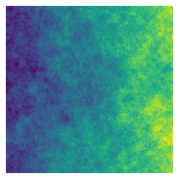
A gradient with noise, cut into three classes: a land cover that changes along a climate.

Model file (TOML)

format = "terraflux/1"

[[nodes]]
id = "gradient"
op = "nlm.planar_gradient"
params = { rows = 200, columns = 200, direction = 90 }

[[nodes]]
id = "noise"
op = "nlm.fbm"
params = { rows = 200, columns = 200, dimension = 1.2, seed = 5 }

[[nodes]]
id = "merged"
op = "nlm.merge"
inputs = { primary = "gradient.map", secondary = "noise.map" }
params = { scaling = 0.8 }
note = "The gradient plus 0.8 times the noise, rescaled to 0-1."

[[nodes]]
id = "classes"
op = "nlm.classify"
inputs = { map = "merged.map" }
params = { weights = [0.5, 0.3, 0.2] }
note = "Classes 1, 2, 3 of 50, 30 and 20% of the cells."

nlm.merge takes the main surface on primary and one or more on secondary; the scaling weighs the secondary ones, so 0.8 keeps the gradient visible under the noise. nlm.classify's output is classes; with its input real connected to a real map, it takes the shares of that map's classes (part 2 uses it).

Common pitfalls#

One map is not an answer. A neutral landscape is one draw; a conclusion needs replicates (different seeds) and their spread (part 2).
Forgetting the cell size. Without resolution, a cell is 1 unit wide: metrics in hectares are then meaningless. Give the cell size of the real maps you compare with.
Comparing amounts that drift. Random clusters and percolation give approximately the share asked for; cut a surface with nlm.binarize when the amount must be exact.
Random cluster above the threshold, above.
Reading a neutral pattern as realistic. Fractal surfaces have no roads, rivers or straight field boundaries; real landscapes made by people are often more regular than any of these models.
The same seed everywhere. Two nodes with the same seed and settings draw the same map: vary the seeds of replicates, and of nodes that should be independent.

Going further#

Part 2: neutral landscapes as an experiment and as a null model, with replicates.
Landscape metrics: measuring the patterns drawn here.
Fragmentation: habitat loss and fragmentation, and the thresholds of real landscapes.
The operator reference: nlm.random, nlm.percolation, nlm.random_cluster, nlm.fbm, nlm.gaussian_field, nlm.mpd, nlm.binarize, nlm.classify, nlm.merge.

References#

Etherington, T. R., Holland, E. P., & O'Sullivan, D. (2015). NLMpy: a Python software package for the creation of neutral landscape models within a general numerical framework. Methods in Ecology and Evolution, 6(2), 164–168. https://doi.org/10.1111/2041-210X.12308
Fahrig, L. (2003). Effects of habitat fragmentation on biodiversity. Annual Review of Ecology, Evolution, and Systematics, 34, 487–515. https://doi.org/10.1146/annurev.ecolsys.34.011802.132419
Gardner, R. H., Milne, B. T., Turner, M. G., & O'Neill, R. V. (1987). Neutral models for the analysis of broad-scale landscape pattern. Landscape Ecology, 1(1), 19–28. https://doi.org/10.1007/BF02275262
Keitt, T. H. (2000). Spectral representation of neutral landscapes. Landscape Ecology, 15(5), 479–494. https://doi.org/10.1023/A:1008193015770
Palmer, M. W. (1992). The coexistence of species in fractal landscapes. The American Naturalist, 139(2), 375–397. https://doi.org/10.1086/285332
Saura, S., & Martínez-Millán, J. (2000). Landscape patterns simulation with a modified random clusters method. Landscape Ecology, 15(7), 661–678. https://doi.org/10.1023/A:1008107902848
Sciaini, M., Fritsch, M., Scherer, C., & Simpkins, C. E. (2018). NLMR and landscapetools: an integrated environment for simulating and modifying neutral landscape models in R. Methods in Ecology and Evolution, 9(11), 2240–2248. https://doi.org/10.1111/2041-210X.13076
Stauffer, D., & Aharony, A. (1994). Introduction to percolation theory (2^nd ed.). Taylor & Francis.
With, K. A. (1997). The application of neutral landscape models in conservation biology. Conservation Biology, 11(5), 1069–1080. https://doi.org/10.1046/j.1523-1739.1997.96210.x
With, K. A., & Crist, T. O. (1995). Critical thresholds in species' responses to landscape structure. Ecology, 76(8), 2446–2459. https://doi.org/10.2307/2265819