A cellular automaton by hand

Before using a model as rich as Dinamica EGO's, it helps to write a simulation whose every rule you know. In this part you will build a cellular automaton of a city that grows: a loop that, at every time step, turns into city the cells that touch the city and are suited to it. It takes ten nodes and runs in a fraction of a second. At the end you will know how Terraflux runs a simulation (a control.repeat loop that carries a map from step to step), how a neighbourhood rule shapes what the simulation draws, and why the shape of simulated patches is something to look at, not a detail.

The idea#

A cellular automaton is a grid of cells, each in a state, updated in time steps by rules that look at the cell and at its neighbourhood (part 1 of this series). Here the states are two, city (1) and not city (0), and the rule is one:

Key idea: the rule of the automaton

At step \(t+1\), a cell \(i\) becomes city if, at step \(t\),

\[ c_i = 0 \quad\text{and}\quad \sum_{j \in N(i)} c_j \ge k \quad\text{and}\quad s_i > s_0 - b\,t \]

where \(c_i\) is 1 when the cell is city and 0 otherwise, \(N(i)\) is the 3 × 3 window around the cell (its 8 neighbours; the cell itself adds 0, since it is not city), \(k\) the number of city neighbours needed (here 2), \(s_i\) the cell's suitability for a city (0 to 1), \(s_0\) the suitability needed at the start (0.6) and \(b\) how much that bar falls every step (0.004). A cell that is city stays city.

The rule has the three ingredients of most land change models in miniature. The neighbourhood term makes the city grow from its edges, not anywhere. The suitability term (the where of part 1) makes it grow first into the attractive land near the centre. And the falling bar plays the role of the quantity: as time goes on, less suited land is accepted, and the city grows faster. The rule is deterministic: run it twice and you get the same city. Dinamica EGO's rules, in the next series, are probabilities drawn at random.

The rule applied to a small grid — The rule on a toy grid. Left: the city at step t. Middle: for every cell, the city cells in its 3 × 3 window (nbsum(c == 1, 1)); the orange square is the window of one cell. Right: at step t + 1, the cells that were not city and had at least 2 city cells around them have become city (light).

Cellular automata of cities have a long history. White and Engelen (1993) grew cities with fractal edges like those of real ones from a few such rules; Clarke et al. (1997) calibrated a CA with rules for spontaneous, edge and road-influenced growth on a century of maps of the San Francisco Bay Area (the model later known as SLEUTH). The rule here is far simpler than theirs, but it is enough to see what a neighbourhood does.

When to use it#

A hand-written automaton is for learning and for testing ideas: what a rule does to the pattern of change, how sensitive a result is to a threshold, what a scenario of "growth only near roads" looks like. It is also how you add a process the classic models lack (a rule of succession, a fire, a protected zone) inside a bigger model, since the same loop holds Dinamica EGO's nodes. It is not a calibrated model of a real place: its rules are guesses. To learn the rules from maps of the past, use the models of the next series (Dinamica EGO's weights of evidence and Expander and Patcher), or CLUE-S and PLUS.

What you need#

Nothing: the template A city that grows (a loop) draws its own landscape with neutral landscape models (maps drawn by chance, with the spatial structure asked for), so it runs as soon as it opens. With your own data, a raster.read of an elevation model, of a map of attractiveness (distance to jobs, to roads) and of the existing city replaces the drawn maps.

This page's bar and the template's

The template asks for three city neighbours and lowers its bar from 0.6 by 0.008 a step over 25 steps. This page asks for two and lowers it by 0.004 over 40 steps, a slower city: edit the expression of the node grow and the loop's times as shown below. Whatever the rule, a bar above all the land within reach of the city (try starting it at 0.8: the cells around the old town have a suitability of 0.50 to 0.59) is a rule that is never true, and the first thing to look for when a simulation does not move.

Build the model#

The landscape#

The landscape: a relief, how attractive each place is, the distance to the old town, and from them the suitability and the city at the start.

Model file (TOML)

format = "terraflux/1"

[[nodes]]
id = "relief"
op = "nlm.gaussian_field"
params = { rows = 150, columns = 150, range = 30, nugget = 0, seed = 41 }
note = "A relief from 0 to 1 (in its place, a raster.read of an elevation model)."

[[nodes]]
id = "attraction"
op = "nlm.gaussian_field"
params = { rows = 150, columns = 150, range = 20, seed = 42 }
note = "How attractive each place is (the jobs, the roads...): 0 to 1."

[[nodes]]
id = "centre"
op = "nlm.distance_gradient"
params = { rows = 150, columns = 150, origin = [72, 78, 72, 78], nlmr_compat = false, rescale = false }
note = "The distance to the old town in the middle."

[[nodes]]
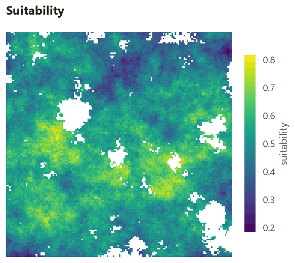
id = "suitability"
op = "raster.calc"
inputs = { a = "attraction.map", d = "centre.map", r = "relief.map" }
params = { expression = "None if r < 0.3 or r > 0.75 else 0.6 * a + 0.4 * (1 - d / 106)" }
note = "Where a city would rather grow: attractive and near the centre; no value (never) in the water and on the mountains."

[[nodes]]
id = "town"
op = "raster.calc"
inputs = { d = "centre.map", suit = "suitability.map" }
params = { expression = "None if isnull(suit) else d == 0" }
note = "The city at the start: the old town (1), the rest 0."

Open the template. In the application, Templates (in groups: Land change) → A city that grows (a loop). It runs at once; its nodes appear in the Model pane and the Viewer opens its last Plot. Its other Plots are in the Viewer's Plots menu.
A relief (node 1): nlm.gaussian_field draws a smooth random surface of 150 × 150 cells, whose values change over about range = 30 cells. Its lowest land will be water and its highest mountains: no city there.
Attraction (node 2): another random surface, with a shorter range (20 cells), standing for jobs, roads and services.
The centre (node 3): nlm.distance_gradient gives each cell its distance (in cells) to the rectangle of rows and columns 72 to 78, the old town.
Suitability (node 4): raster.calc combines them: 60% attraction and 40% nearness to the centre (the distance divided by 106, the largest distance on the map). Water (relief below 0.3) and mountains (above 0.75) get None, a missing value: a cell without a value never changes.
The town (node 5): d == 0 is 1 in the old town and 0 elsewhere; cells of water or mountain stay missing.

The suitability of the landscape for the city — The suitability: high (yellow) in attractive land near the centre; blank cells are water and mountains, where the city never goes.

The loop#

A simulation is a loop: the map of each step is computed from the map of the step before. In Terraflux this is a control.repeat node, a container whose body is a small model of its own, run once per step.

The loop: control.repeat runs its body 40 times; the body turns into city the suited cells next to the city. carry passes the city from step to step, collect keeps every step's map.

Model file (TOML)

format = "terraflux/1"

[[nodes]]
id = "growth"
op = "control.repeat"
inputs = { times = 40, city = "town.map" }
note = "Every step its body runs with @city, the city of the step before, and @step."

[nodes.body]
carry = { city = "grow.map" }
collect = { maps = "grow.map" }

[[nodes.body.nodes]]
id = "grow"
op = "raster.calc"
inputs = { c = "@city", suit = "suitability.map", step = "@step" }
params = { expression = "1 if c == 0 and nbsum(c == 1, 1) >= 2 and suit > 0.6 - step * 0.004 else c" }
note = "A cell becomes city when two of its neighbours are, if it is suited enough; the bar falls a little every step."

The loop's settings are the heart of every simulation in Terraflux, Dinamica EGO's included:

times = 40: how many steps. Here a step has no unit; in a calibrated model it is a year, or the time between two maps divided into steps.
city = "town.map": an input of any name becomes a carried value. At step 1, @city inside the body is the town; at every later step it is the value of its carry reference at the end of the step before.
carry = { city = "grow.map" }: what @city becomes for the next step: the map the body just made.
collect = { maps = "grow.map" }: a series, the map of every step, given out as growth.maps (40 maps). The carried value after the last step is growth.city.
@step is the number of the step (1 to 40), used here to lower the bar.

Inside the body, grow reads @city, @step and suitability.map, a node outside the loop: a body can read any node of the model, and what does not depend on the step is computed once. nbsum(c == 1, 1) is the sum, over the square of radius 1 (3 × 3 cells) around each cell, of c == 1 (1 for city, 0 otherwise): the number of city cells around it.

In the application

Double-click the growth node (or Open inside in the Node pane) to edit its body; the trail at the top of the canvas takes you back. Inside, the column on the left lists what the body can read: @city, @step and the outer nodes. Select grow and edit its expression in the Node pane; Ctrl+Enter runs the model to the node selected. The template's Plots show growth.maps (a slider over the steps) and growth.city.

The whole model, as the application shows it:

A city that grows, with this page's bar and 40 steps: the landscape (nodes 1 to 5) and the loop with its body (node 6). The template keeps three Plots: the city step by step (growth.maps), the last city (growth.city) and the suitability.

Model file (TOML)

format = "terraflux/1"
name = "A city that grows (a loop)"

[[nodes]]
id = "relief"
op = "nlm.gaussian_field"
params = { rows = 150, columns = 150, range = 30, nugget = 0, seed = 41 }

[[nodes]]
id = "attraction"
op = "nlm.gaussian_field"
params = { rows = 150, columns = 150, range = 20, seed = 42 }

[[nodes]]
id = "centre"
op = "nlm.distance_gradient"
params = { rows = 150, columns = 150, origin = [72, 78, 72, 78], nlmr_compat = false, rescale = false }

[[nodes]]
id = "suitability"
op = "raster.calc"
inputs = { a = "attraction.map", d = "centre.map", r = "relief.map" }
params = { expression = "None if r < 0.3 or r > 0.75 else 0.6 * a + 0.4 * (1 - d / 106)" }

[[nodes]]
id = "town"
op = "raster.calc"
inputs = { d = "centre.map", suit = "suitability.map" }
params = { expression = "None if isnull(suit) else d == 0" }

[[nodes]]
id = "growth"
op = "control.repeat"
inputs = { times = 40, city = "town.map" }

[nodes.body]
carry = { city = "grow.map" }
collect = { maps = "grow.map" }

[[nodes.body.nodes]]
id = "grow"
op = "raster.calc"
inputs = { c = "@city", suit = "suitability.map", step = "@step" }
params = { expression = "1 if c == 0 and nbsum(c == 1, 1) >= 2 and suit > 0.6 - step * 0.004 else c" }

[[plots]]
id = "plot_growth"
title = "The city, step by step"
layers = [{ from = "growth.maps" }]

[[plots]]
id = "plot_city"
title = "The city after 25 steps"
layers = [{ from = "growth.city" }]

[[plots]]
id = "plot_suitability"
title = "Suitability"
layers = [{ from = "suitability.map" }]

From the command line, the same model saved as city.toml runs with terraflux run city.toml. Plots write nothing; to keep the maps, add a raster.write node whose value is growth.maps (a GeoTIFF with a band per step) or an output of the model:

[outputs.city]
from = "growth.maps"

Read the results#

Move the slider, or press play, to watch the city grow. The chart beside it follows the slider: the share of the land (the cells that are neither water nor mountain) that is city. Save as GIF..., under the slider, saves the growth as an animation (each step written in its corner, the legend under the map) to show in a talk, at the speed chosen above it; Save as MP4... saves it as a video.

Step 2 — The city every two steps (city in purple, open land in beige, water in blue, mountains in grey). Slow at first, while only the best land passes the bar, then faster as the bar falls and the edge grows longer.

Three things are worth seeing in this run.

The growth curve. The city covers 0.2% of the land or less for the first ten steps and 7.2% at step 40, with most of the growth after step 20. Nothing in the rule says "accelerate": the acceleration comes from the bar falling (more land qualifies) and from the edge getting longer (more cells have city neighbours). Simulations often produce curves like this by themselves, which is why the quantity of change is usually imposed from outside (a demand, a rate), as the models of the next series do, rather than left to the rules.

The shape. The city grows as a diamond with straight edges at 45°. That shape is not in the landscape: it is the neighbourhood. With a rule of two neighbours in a 3 × 3 window, a front moves at most one cell per step, and faster along the diagonals than along the rows. A geometric shape in a simulated map is a sign that the rule, not the landscape, is deciding where change goes.

The limits. The city stops at the water (blue) and leaves holes where the suitability is low: the suitability does constrain it, but only at its edge.

Settings that change the answer#

The number of city neighbours a cell needs, \(k\), changes the city completely. Each image is the city after 40 steps of the same model with another \(k\):

With \(k = 1\) any cell touching the city may join, and the front advances one cell per step in all eight directions: a square. With \(k = 4\) almost no cell outside a convex city has four city neighbours, and the city never leaves the old town. Between them, the city's area after 40 steps varies by a factor of almost 90, for the same landscape and the same suitability. The other settings act in the same way: \(s_0\) and \(b\) set how fast suitability stops being a barrier; times sets how far a front can go (at most one cell per step here).

This is the main lesson of this part, and it holds for every model in this series: the rules that place change decide the pattern of the simulated landscape as much as the drivers do. Dinamica EGO's patches, CLUE-S's competition and PLUS's seeds are, each, a more refined answer to the same question this \(k\) answers. Before trusting a simulated map, look at its patches: their sizes, their shapes, their distance from existing ones.

Common pitfalls#

nbcount is not a count of true cells. The rule counts the city neighbours with nbsum(c == 1, 1): c == 1 is 1 on a city cell and 0 elsewhere, so the sum is the number of city cells. nbcount(x, r) counts something else, the cells with a value in the window (it is for averages over the cells with data), so nbcount(c == 1, 1) >= 2 is true for almost every cell. Written that way, the rule lets the city appear wherever the suitability passes the bar, far from the town: 81.6% of the land is city after 40 steps. To count the cells where a condition holds, use nbsum(condition, r); for the share of them, nbmean(condition, r).

The city after 40 steps when the rule uses nbcount — The same model with nbcount(c == 1, 1) >= 2 in place of nbsum: the neighbour test always passes and the city covers 81.6% of the land, wherever the suitability allows.

Synchronous updates. Every cell of a step reads the map of the step before, so a city can grow at most r cells per step. A rule that seems to "stop" may only need more steps.
Missing values spread. Any arithmetic with a missing value gives a missing value. Here water and mountains are missing on purpose; a driver missing by mistake (a gap in an elevation model) makes cells that never change. Neighbourhood functions leave missing cells out.
Edges of the map. At the border a window has fewer cells, and a rule on counts behaves differently there. Keep a margin around the study area, or use shares (nbmean) instead of counts.
A rule fitted to nothing. The thresholds here are guesses. A model meant to say something about a real place needs its rules estimated from observed change (the next series) and checked against a period it has not seen (the third).

Going further#

Transition rates with Markov chains: the next part, how much changes per step when it is learned from two maps.
Building models: map algebra, loops, groups and submodels in depth.
The loop of Dinamica EGO's model is this same control.repeat with two nodes in its body.
The operators: control.repeat, raster.calc, nlm.gaussian_field, nlm.distance_gradient.

References#

Clarke, K. C., Hoppen, S., & Gaydos, L. (1997). A self-modifying cellular automaton model of historical urbanization in the San Francisco Bay area. Environment and Planning B: Planning and Design, 24(2), 247–261. https://doi.org/10.1068/b240247
Soares-Filho, B. S., Coutinho Cerqueira, G., & Lopes Pennachin, C. (2002). DINAMICA: a stochastic cellular automata model designed to simulate the landscape dynamics in an Amazonian colonization frontier. Ecological Modelling, 154(3), 217–235. https://doi.org/10.1016/S0304-3800(02)00059-5
White, R., & Engelen, G. (1993). Cellular automata and fractal urban form: a cellular modelling approach to the evolution of urban land-use patterns. Environment and Planning A, 25(8), 1175–1199. https://doi.org/10.1068/a251175